| Transition Temperature | 125 K |
|---|---|
| Experiment Temperature | 2 K |
| Propagation Vector | k1 (0, 0, 0) |
| Parent Space Group | Pnma (#62) |
| Magnetic Space Group | P212121 (#19.25) |
| Magnetic Point Group | 222 (6.1.17) |
| Lattice Parameters | 9.75990 5.75190 4.75600 90.00 90.00 90.00 |
|---|---|
| DOI | 10.1021/cm0300462 |
| Reference | G. Rousse, J. Rodriguez-Carvajal, S. Patoux and C. Masquelier, Chemistry of Materials (2003) 15 4082-4090. |
| Label | Element | Mx | My | Mz | |M| |
|---|---|---|---|---|---|
| Fe1 | Fe | 4.06 | 0.9 | 0.0 | 4.16 |
Magnetic Structures of the Triphylite LiFePO_{4} and of Its Delithiated Form FePO_{4}
G. Rousse \( ^{*} \)
Institut Laue Langevin, BP 156, F-38042 Grenoble Cedex 9, France, and Physique des Milieux Condensés, Université P. et M. Curie, 4 place Jussieu, 75252 Paris Cedex 05, France
J. Rodriguez-Carvajal
Laboratoire Léon Brillouin (CEA-CNRS), CEA/Saclay, 91191 Gif sur Yvette Cedex, France, and Service de Physique Statistique, CEA/Grenoble, 17 Avenue des Martyrs, 38054 Grenoble Cedex 9, France
S. Patoux and C. Masquelier \( ^{*} \)
Laboratoire de Réactivité et Chimie des Solides, Université Picardie Jules Verne, 33 Rue St. Leu, 80039 Amiens Cedex 9, France
Received February 6, 2003. Revised Manuscript Received July 17, 2003
The magnetic structures of \( LiFePO_{4} \) and of its delithiated form \( FePO_{4} \) (triphylite, olivine group, space group Pnma) have been solved using neutron diffraction on polycrystalline samples. Both compounds show antiferromagnetic behavior below 52 K for \( LiFePO_{4} \) ( \( Fe^{2+} \) ) and below 125 K for \( FePO_{4} \) ( \( Fe^{3+} \) ), characterized by the appearance of extra peaks in the neutron diffraction patterns below the Néel temperature. These magnetic reflections are indexed with a propagation vector \( \mathbf{k} = (0,0,0) \) . The magnetic moments of the four iron atoms present in the unit cell are oriented along [010] for \( LiFePO_{4} \) and mostly along [100] (with a small component along [010]) for \( FePO_{4} \) . The magnetic structures and the differences in the Néel temperatures are discussed in terms of super and super-super exchange interactions and of anisotropy of \( Fe^{2+} \) . A comparison is made with other olivine compounds with similar cation distribution.
Introduction
LiFePO_{4} (triphyllite) is one of the members of the olivine family, with Li on the M1 site (4a, on the inversion center) and Fe on the M2 site (4c, on the mirror plane) of space group Pnma. Triphyllite has been the subject of intense research over the past 3 years as it is a very promising compound for use as a Li-ion positive electrode. \( ^{1} \) One can indeed reversibly remove Li ions from it, leading to a crystalline form of the composition FePO_{4}. This new phase, which retains the olivine structure, is to our knowledge the only olivine-type compound into which the M1 site is empty. Exceptions are minerals of formulas Fe_{1-x} Mn_{x}PO_{4} (x \sim \( \frac{1}{3} \) heterosite and x \sim \( \frac{2}{3} \) purpurite), which usually present disorder and impurities due to their natural origin and solid solution character.
Many other compounds adopt the olivine structure and have been widely studied for their magnetic properties. The principal interest in the olivine structure is that it presents frustration effects. \( ^{2} \) However, most of these studies concern olivine compounds for which the magnetic ion (Fe, Mn, Co) lies on the M1 and the M2 sites (Mn \( _{2} \) SiS \( _{4} \) or Fe \( _{2} \) SiS \( _{4} \) \( ^{3} \) ) or on the M1 site only (NaCoPO \( _{4} \) , NaMnPO \( _{4} \) , NaFePO \( _{4} \) \( ^{4,5} \) ). We are interested here in two olivine compounds for which only the M2 site is occupied by a magnetic ion. LiFePO \( _{4} \) presents the same structure as the magnetoelectric compounds LiNiPO \( _{4} \) and LiCoPO \( _{4} \) whose magnetic structures are known. \( ^{6-8} \) It is isostructural with LiMnPO \( _{4} \) as well, whose magnetic structure was determined in the early 1960s. \( ^{9,10} \) Santoro and Newman have also reported the magnetic structure of LiFePO \( _{4} \) . \( ^{11} \) If the magnetic structures of the transition metal olivines are often complex, those of LiMnPO \( _{4} \) , LiCoPO \( _{4} \) , LiNiPO \( _{4} \) , and LiFePO \( _{4} \) are reported to be all collinear, but with different spin orientations.
In such a context, it was tempting to compare the magnetic behavior of LiFePO \( _{4} \) and FePO \( _{4} \) , which present both the olivine structure with the magnetic ions on the M2 site (4c), and investigate whether the structures

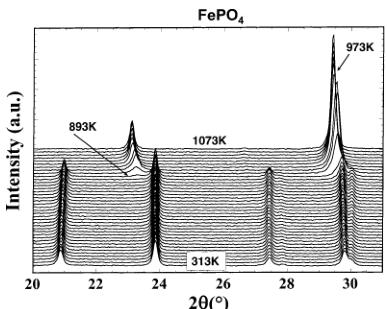
Figure 1. Thermal evolution of triphyllite \( FePO_{4} \) recorded on a D8 Bruker diffractometer (Co Kα)–geometry, PSD counter. The sample was placed in an Anton Parr chamber (ATK1200) and heated at 0.5°/min in increments of 20 K between 313 and 1073 K. At each temperature, kept stable, the XRD pattern was recorded within \( \approx \) 20 min.
obtained will be collinear despite the possible geometric frustration due to the presence of triangular platelets in the structure. The only differences between these two compounds is that chemical extraction of \( Li^{+} \) from \( LiFe^{II}PO_{4} \) results in oxidation of \( Fe^{2+} \) into \( Fe^{3+} \) and hence to lattice parameters contractions in \( Fe^{III}PO_{4} \) (along the a and b axis (respectively, -5.6% and -4.3%), the c lattice parameter being slightly increased by +1.5%). Additionally, the M1 site (4a) is empty for \( FePO_{4} \) .
Experimental Section
Pure LiFePO_{4} was prepared as described elsewhere \( ^{12} \) as fine and dispersed fine particles (<500 nm) with a specific surface area of 3 m^{2}/g. FePO_{4} was easily obtained by chemical extraction of lithium from LiFePO_{4}: 5 g of LiFePO_{4} powder was dispersed into an acetonitrile solution of NO_{2}BF_{4} under air at 80 °C (reflux) for a week. The resulting solid was washed several times with acetonitrile and dried under vacuum. Note that this unusual form of FePO_{4} is stable in air until 893 K, at which temperature it transforms irreversibly into the low-temperature form (a) of FePO_{4} quartz (Figure 1). Between 293 and 893 K, the behavior of the unit-cell parameters, refined by the Rietveld method using the X-ray data shown in Figure 1, reveals a global isotropic expansion \( \Delta V/V = 5\% \) ( \( \Delta a/a = 1.2\% \) ; \( \Delta b/b = 2\% \) ; \( \Delta c/c = 1.8\% \) ). Figure 1 shows, additionally, the well-known \( \alpha \leftrightarrow \beta \) transition of FePO_{4} quartz at 973 K, as reported by Shafer et al. \( ^{13} \)
Neutron diffraction experiments were performed at the Institute Laue Langevin (ILL, Grenoble, France), on the high-intensity powder diffractometer D20, at wavelengths of 2.41 Å (obtained by a HOPG graphite monochromator) and of 1.30 Å (obtained by a copper monochromator). The powdered sample (a few tens of milligrams in the case of \( FePO_{4} \) ) was placed inside a vanadium can mounted on a cryostat. The diffractometer D20 has been used in its normal high-flux configuration for measuring the sample between 2 and 300 K (primary divergence of 27°). In the case of \( LiFePO_{4} \) , for which a larger amount of powder was available, a primary divergence of 10' and vertical monochromator windows of 15 mm were used to increase the resolution of the instrument. The program FullProf \( ^{14} \) was used for crystal and magnetic structure refinements using the Rietveld method \( ^{15} \) and for distance and bond valence sum calculations. \( ^{16} \)

(a)

(b)
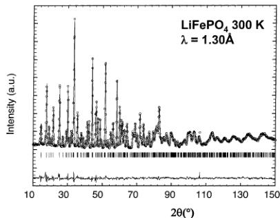
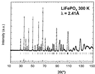
Figure 2. Calculated (continuous line) and experimental (circles) neutron diffraction patterns of \( LiFePO_{4} \) at 300 K at a wavelength of 1.30 Å (Figure 2a) and 2.41 Å (Figure 2b) (D20 data).
Results and Discussion
(a) Nuclear Structure of LiFePO₄ at 300 K. The nuclear structure of our sample of LiFePO₄ has been checked by a simultaneous Rietveld refinement of two sets of neutron data recorded at 1.30 and 2.41 Å, respectively, from the structure published by Santoro. \( ^{[11]} \) The final refinements are shown in Figure 2a,b. The structure of triphyllite LiFePO₄ is described in the orthorhombic space group Pnma (a = 10.338(1) Å, b = 6.011(1) Å, c = 4.695(1) Å). The major part of the atoms are distributed in the special position 4c; the exceptions are Li in the 4a position (on the inversion center) and O(3), which lies in the general position 8d (Table 1). There is only a single crystallographic site for Fe atoms (4c, on a mirror plane), located at the middle of a slightly distorted FeO₆ octahedron, with Fe–O distances ranging from 2.06(2) to 2.25(3) Å, as can be seen in Table 2. The average Fe–O distance is higher than what is expected for iron in the +2 valence state in octahedral coordination, probably due to the fact that the FeO₆ octahedron shares edges with PO₄ tetrahedra. Electrostatic repulsions between Fe and P ions weaken the
Table 1. Structural Parameters of LiFePO₄ (Pnma) Determined from Neutron Diffraction at 300 K (Combined Refinement from Data Recorded with 1.30 and 2.41 Å Wavelengths); Atomic Positions of the Magnetic Ions in the Unit Cell and Their Magnetic Moment (μB) at 2 K Are Given
| LiFePO4, D20 at 300 K: Space Group Pnma | ||||
| a = 10.3377(5) Å, b = 6.0112(2) Å, c = 4.6950(2) Å | ||||
| atom | x | y | z | Biso(Å2) |
| Li | 0 | 0 | 0 | 1.3(2) |
| Fe | 0.2822(2) | 1/4 | 0.9738(5) | 0.55(5) |
| P | 0.0950(3) | 1/4 | 0.418(6) | 0.3(1) |
| O(1) | 0.09713(3) | 1/4 | 0.7428(7) | 0.69(5) |
| O(2) | 0.4573(3) | 1/4 | 0.2067(7) | 0.69(5) |
| O(3) | 0.166(3) | 0.0464(4) | 0.2851(4) | 0.69(5) |
Magnetic Moments ( \( \mu_{B} \) ) at 2 K
| atom | x | y | z | M_{X} | M_{Y} | M_{Z} |
| Fel | 0.2822 | \( ^{1}/_{4} \) | 0.9738 | 0 | 4.19(5) | 0 |
| Fe2 | 0.2178 | \( ^{3}/_{4} \) | 0.4738 | 0 | -4.19(5) | 0 |
| Fe3 | 0.7178 | \( ^{3}/_{4} \) | 0.0262 | 0 | -4.19(5) | 0 |
| Fel4 | 0.7822 | \( ^{1}/_{4} \) | 0.5626 | 0 | 4.19(5) | 0 |
Table 2. Iron Environment in LiFe \( ^{II} \) PO \( _{4} \) and Fe \( ^{III} \) PO \( _{4} \) : Fe–O Distances, Average Distance, and Distortion \( \Delta \) of the Polyhedra Are Reported; Distortion Parameter \( \Delta \) for a Coordination Polyhedron BO \( _{N} \) Is Defined As \( \Delta = (1/N)\sum_{n=1,N}\{(d_{n} - \langle d \rangle)/(d)\}^{2} \) If \( \langle d \rangle \) Is the Average B–O Distance
| LiFePO4 | FePO4 |
| Fe-O(I): 2.199(4) Å | Fe-O(I): 1.890(3) Å |
| Fe-O(2): 2.115(4) Å | Fe-O(2): 1.909(3) Å |
| 2 × Fe-O(3): 2.253(3) Å | 2 × Fe-O(3): 2.133(2) Å |
| 2 × Fe-O(3): 2.061(2) Å | 2 × Fe-O(3): 2.011(2) Å |
| average distance: 2.157(1) Å | average distance: 2.015(1) Å |
| predicted average | predicted average |
| distance: 2.1405 Å | distance: 2.0155 Å |
| bond valence sum \( ^{16} \) : 1.96(1) | bond valence sum \( ^{16} \) : 3.10(1) |
| distortion: \( \Delta = 14.6 \times 10^{-4} \) | distortion: \( \Delta = 22.5 \times 10^{-4} \) |
Fe–O bond strength, which is at the origin of the unusually high operating voltage vs \( Li^{+}/Li \) of this electrode material when lithium ions are extracted from the framework (3.45 V vs \( Li^{+}/Li \) ). \( ^{17} \)
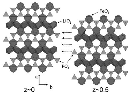
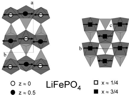
A simple way to describe the triphlyite structure of \( LiFePO_{4} \) is to establish a parallel between the olivine family (to which \( LiFePO_{4} \) belongs) and the spinel family. Both spinel and olivine structures correspond to a structural formula \( AB_{2}O_{4} \) where A and B occupy tetrahedral and octahedral cavities respectively of O close packing: cubic in the case of spinel and hexagonal in the case of olivine. In the case of spinel, there are two types of cation distributions between dense oxygen layers that alternate perpendicular to the [111]cubic direction: \( Oc_{3} \) layers ("Kagomé") where \( ^{3}/_{4} \) of the octahedral sites are filled and \( Te_{2}Oc \) layers where \( ^{1}/_{4} \) of the octahedral sites are filled and \( ^{2}/_{8} \) of the tetrahedral sites are filled. In the case of olivine, there is only one type of cation distribution, \( TeOc_{2} \) , between dense oxygen layers, that is repeated perpendicular to the [001] hexagonal direction. In the case of \( LiFePO_{4} \) , Figure 3 shows that Li and Fe are distributed within the octahedral sites in a very different manner. Within one \( TeOc_{2} \) layer (where \( ^{1}/_{2} \) of the octahedral sites are filled and \( ^{1}/_{8} \) of the tetrahedral sites are filled), Li is distributed to form \( LiO_{6} \) chains sharing edges and running parallel to [010] \( _{ortho} \) , while Fe is distributed so as to form \( FeO_{6} \) octahedra isolated from each other. Figure 3 also illustrates the two-dimensional character of

Figure 3. Two \( TeOc_{2} \) layers at \( z \sim 0 \) (left) and \( z \sim 0.5 \) (right) of the triphyllite structure showing the \( LiO_{6} \) octahedral chains that when the layers are superimposed (following the dotted arrows) are not in contact. The voids between \( FeO_{6} \) octahedra along [010] in one layer at \( z \sim 0 \) are filled by the next one at \( z \sim 0.5 \) through corner sharing.

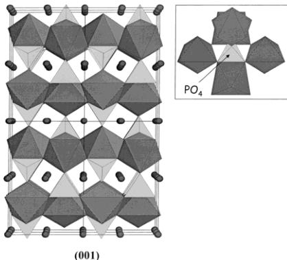
Figure 4. General view of LiFePO₄. Tunnels via which lithium ions can be removed can be seen in the [010] and [001] directions. Inset: PO₄ tetrahedron connected to five FeO₆ octahedra.
LiFePO_{4} as a second TeOc_{2} layer comes at the vertical of the previous one, to build (100) layers of FeO_{6} octahedra sharing corners and (100) mixed layers of LiO_{6} octahedra and PO_{4} tetrahedra.
Each \( FeO_{6} \) octahedron is connected to four other \( FeO_{6} \) octahedra via vertices, and to four \( PO_{4} \) tetrahedra, one of them being connected via an edge. Vice versa, each \( PO_{4} \) tetrahedron is connected to five \( FeO_{6} \) octahedra, one of them sharing an edge (Figure 4). A more general view of the structure is given in Figure 4, where tunnels via which lithium ions can be removed are clearly identified in the [010] and [001] directions.
(b) Extraction of Lithium from LiFePO_{4}-Nuclear Structure of FePO_{4} at 300 K. Using a classical oxidative reaction (see Experimental Section), we easily obtained the delithiated form, FePO_{4}, of triphyllite LiFePO_{4} where the respective positions of Fe and P atoms are essentially unchanged. The extraction of lithium is naturally accompanied, for charge balance, by the oxidation of Fe^{2+} to Fe^{3+} occurring, in an electrochemical cell, at 3.45 V vs Li^{+}/Li.^{17,18} The nuclear

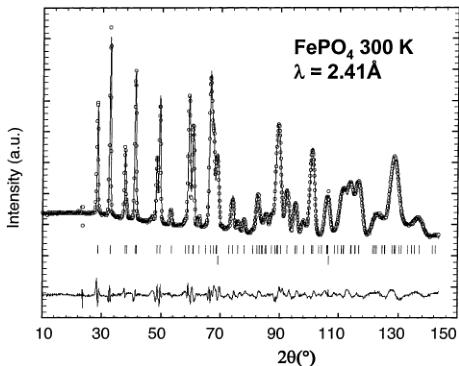
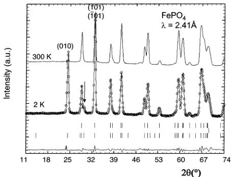
Figure 5. Calculated (continuous line) and experimental (circles) neutron diffraction patterns of \( FePO_{4} \) at 300 K at a wavelength of 2.41 Å (D20 data). The lower sticks indicate Bragg positions of vanadium arising from the container (see text).
structure of \( FePO_{4} \) has been investigated using neutron diffraction data recorded at 300 K ( \( \lambda = 2.41 \, \AA \) ). The handicap of possessing small amounts of powder at the time of our experiment was overcome by the use of the extra high-intensity diffractometer D20: this instrument has a very large microstrips detector (array of 1536 detector cells arranged at \( 0.1^{\circ} \) intervals in \( 2\theta \) , covering the whole \( 2\theta \) range up to \( 155^{\circ} \) ).
The Rietveld refinement of the collected data was performed using the initial list of atomic positions in the nuclear structure, published recently by Andersson and Thomas. \( ^{[19]} \) Note that, in ref 19, the structure was obtained from multiphase neutron powder diffraction data (FePO \( _{4} \) and LiFePO \( _{4} \) ). As we could obtain a pure FePO \( _{4} \) solid, due to the significant overlap between the peaks of LiFePO \( _{4} \) and FePO \( _{4} \) , our refinement should lead to higher accuracy. Note that we added a second “phase” in the refinement to account for the large peak at 69.2° that arises from the vanadium sample container (Im \( \bar{3} \) m, a = 3.011(1) Å). The refinement is shown in Figure 5. The structure of triphytite FePO \( _{4} \) is basically the same as that of LiFePO \( _{4} \) , but with anisotropic lattice parameters variations: contraction along [100] and [010] and, more intriguing, slight elongation along [001]. The lattice parameters of FePO \( _{4} \) are a = 9.760(1) Å, b = 5.752(1) Å, and c = 4.756(1) Å (Table 3), in good agreement with previously reported values. \( ^{[19]} \) As for LiFePO \( _{4} \) , the unique Fe atom is located at the middle of an FeO \( _{6} \) octahedron, which is more distorted than in LiFePO \( _{4} \) (Table 2). The Fe–O distances range from 1.89(1) to 2.13(1) Å, with an average distance of 2.015(1) Å, in good agreement with the expected value for iron in the oxidation state +3 (Table 2).
(c) Magnetic Structures of LiFePO_{4} and FePO_{4}. In this section we present the description of the magnetic structures of LiFePO_{4} and FePO_{4} that were obtained from Rietveld refinements of temperature-
Table 3. Structural Parameters of FePO₄ Determined from Neutron Diffraction at 300 K (Pnma); Atomic Positions of the Magnetic Ions in the Unit Cell and Their Magnetic Moment (μB) at 2 K Are Given
| FePO_{4}, D20 ( \( \lambda = 2.41 \text{ Å} \) ) at 300 K: Space Group Pnma | |||||
| a = 9.7599(8) Å, b = 5.7519(5) Å, c = 4.7560(4) Å | |||||
| atom | x | y | z | B_{iso} ( \( \textup{\AA}^{2} \) ) | |
| Fe | 0.2755(2) | \( ^{1}/_{4} \) | 0.9482(5) | 0.58(7) | |
| P | 0.0939(6) | \( ^{1}/_{4} \) | 0.395(1) | 0.9(1) | |
| O(1) | 0.1215(4) | \( ^{1}/_{4} \) | 0.7089(8) | 1.2(1) | |
| O(2) | 0.4391(5) | \( ^{1}/_{4} \) | 0.1595(8) | 1.3(1) | |
| O(3) | 0.1660(4) | 0.0449(5) | 0.2498(6) | 0.85(8) | |
Magnetic Moments ( \( \mu_{B} \) ) at 2 K
(Total Magnetic Moment 4.15(3) \( \mu_{B} \) )
| atom | x | y | z | \( M_{X} \) | \( M_{Y} \) | \( M_{Z} \) |
| FeI | 0.2755 | \( ^{1}/_{4} \) | 0.9482 | 4.06(2) | 0.90(6) | 0 |
| Fe2 | 0.2245 | \( ^{3}/_{4} \) | 0.4482 | -4.06(2) | -0.90(6) | 0 |
| Fe3 | 0.7245 | \( ^{3}/_{4} \) | 0.0518 | -4.06(2) | 0.90(6) | 0 |
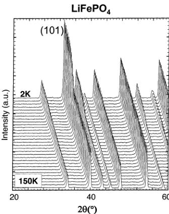
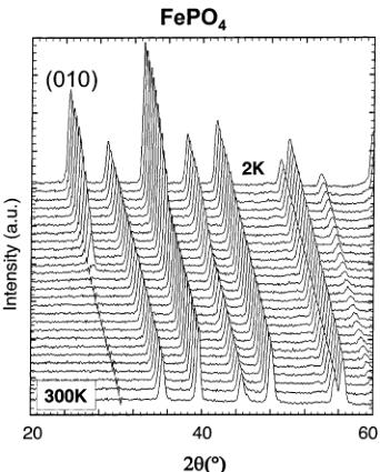
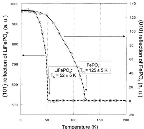
dependent neutron powder diffraction data. As we already mentioned, different magnetic behaviors were expected from these two compounds that differ essentially in the oxidation state of iron (+2 in \( LiFePO_{4} \) , +3 in \( FePO_{4} \) ) and in the occupancy of the octahedral lithium sites 4a (M1 site). On cooling to 2 K, the neutron diffraction patterns of both \( LiFePO_{4} \) and \( FePO_{4} \) show the appearance of some extra reflections (Figure 6). Despite apparent differences between the diffraction patterns of the two compounds, the magnetic reflections of both \( LiFePO_{4} \) and \( FePO_{4}\mathrm{~} \) can be indexed using the propagation vector \( \mathbf{k}=(0,0,0) \) , which indicates that the magnetic unit cell is the same as the nuclear one. However, very different Néel temperatures were found as clearly shown in Figure 7, where we have represented the integrated intensity of the main magnetic reflections ((101) for \( LiFePO_{4} \) ; (010) for \( FePO_{4} \) ) vs temperature. The Néel temperature for \( LiFePO_{4} \) is much lower ( \( T_{N}=52 \) K, in very good agreement with data published by Santoro and Newman \( ^{[1]} \) ) than for \( FePO_{4} \) ( \( T_{N}=125 \) K). As we will discuss later, this difference is probably due to the \( Fe^{3+}-Fe^{3+} \) super and super-super exchange interactions, which are stronger than the \( Fe^{2+}-Fe^{2+} \) interactions. Note also (this will be of importance for the interpretation of the data presented in the following section) that the (010) magnetic reflection is very intense for \( FePO_{4} \) and absent for \( LiFePO_{4} \) , already indicating at first sight that the magnetic structures will not be identical.
As we mentioned earlier, the magnetic centers (Fe) of the cell are distributed over the equivalent positions of the crystallographic site, at the special position 4c, with \( x \approx 0.28 \) , \( y = ^{1}/_{4} \) , \( z \approx 0.96 \) . The different possibilities of magnetic configurations were investigated using Bertaut's symmetry analysis method \( ^{20,21} \) that allows determining the symmetry constraints between magnetic moments of atoms belonging to whatever crystallographic site. We use here the same notations of refs 20 and 21 (see them for details about representations). In the following, we will label as Fe2, Fe3, and Fe4 the three extra iron atoms of the unit cell, deduced from Fe1 (x, y, z) by the symmetry operators: \( (-x + ^{1}/_{2}, -y, \)


Figure 6. Left: Neutron diffraction patterns of \( LiFePO_{4} \) (D20, \( \lambda = 2.41 \AA \) ) between 150 and 2 K, showing the appearance of magnetic peaks below 52 K. Right: Neutron diffraction patterns of \( FePO_{4} \) (D20, \( \lambda = 2.41 \AA \) ) between 300 and 2 K, showing the appearance of magnetic peaks below 125 K.

Figure 7. Evolution of the integrated intensity of the main magnetic reflections for \( LiFePO_{4} \) (101) and for \( FePO_{4} \) (010) as a function of temperature. The NMel temperature for each compound is indicated. The dotted lines are a guide to the eye.
\( z - \frac{1}{2} \) , \( (-x, y + \frac{1}{2}, -z) \) , and \( (x + \frac{1}{2}, -y + \frac{1}{2}, -z + \frac{1}{2}) \) , respectively. The total magnetic representation \( \Gamma \) of the propagation vector group \( (\mathrm{G}_{\mathbf{k}} = \mathrm{Pnma}) \) , for the Wyckoff position 4c, can be decomposed upon eight irreducible representations of dimension 1 as follows:
\[ \Gamma(4\mathbf{c})=\Gamma_{1}+2\Gamma_{2}+2\Gamma_{3}+\Gamma_{4}+\Gamma_{5}+2\Gamma_{6}+2\Gamma_{7}+\Gamma_{8} \]
which leads to eight possible spin configurations, the same for both compounds, described by the basis functions:
\[ \begin{aligned}\Gamma_{1}\colon G^{Y}&=S_{1}^{Y}-S_{2}^{Y}+S_{3}^{Y}-S_{4}^{Y}\\\Gamma_{2}\colon A^{X}&=S_{1}^{X}-S_{2}^{X}-S_{3}^{X}+S_{4}^{X}and\\&\quad C^{Z}=S_{1}^{Z}+S_{2}^{Z}-S_{3}^{Z}-S_{4}^{Z}\end{aligned} \]
\[ \begin{aligned}\Gamma_{3}\colon G^{X}=S_{1}^{X}-S_{2}^{X}+S_{3}^{X}-S_{4}^{X}and\\F^{Z}=S_{1}^{Z}+S_{2}^{Z}+S_{3}^{Z}+S_{4}^{Z}\end{aligned} \]
\[ \Gamma_{4}\colon A^{Y}=S_{1}^{Y}-S_{2}^{Y}-S_{3}^{Y}+S_{4}^{Y} \]
\[ \Gamma_{5}\colon F^{Y}=S_{1}^{Y}+S_{2}^{Y}+S_{3}^{Y}+S_{4}^{Y} \]
\[ \begin{aligned}\Gamma_{6}\colon C^{X}=S_{1}^{X}+S_{2}^{X}-S_{3}^{X}-S_{4}^{X}and\\A^{Z}=S_{1}^{Z}-S_{2}^{Z}-S_{3}^{Z}+S_{4}^{Z}\end{aligned} \]
\[ \Gamma_{7}\colon F^{X}=S_{1}^{X}+S_{2}^{X}+S_{3}^{X}+S_{4}^{X}and\\G^{Z}=S_{1}^{Z}-S_{2}^{Z}+S_{3}^{Z}-S_{4}^{Z} \]
\[ \Gamma_{8}\colon C^{Y}=S_{1}^{Y}+S_{2}^{X}-S_{3}^{Y}-S_{4}^{Y} \]
where \( S_{i}^{X} \) , for instance, is the component along x of the magnetic moment of atom i. The x, y, and z axes are assumed to be along the a, b, and c crystallographic axes. For example, the representation \( \Gamma_{3} \) corresponds to a ferromagnetic coupling of the four Fe atoms of the cell in the z direction, mode \( F^{Z} \) , corresponding to the sequence \( (++++) \) for atoms 1, 2, 3, and 4, whereas in the x direction the moments are coupled antiferromagnetically according to the mode \( G^{X} \) corresponding to the sequence \( (+-+-) \) . We tried all these magnetic models by the Rietveld method on the neutron diffraction data of \( LiFePO_{4} \) and \( FePO_{4} \) recorded at 2 K.
Magnetic Structure of \( LiFePO_{4} \) ( \( Fe^{2+} \) ). Over all the possibilities determined by the symmetry analysis, the collinear solution \( A^{Y} = (+ - - +) \) (antiferromagnetic ordering along [010]) gives the best agreement between observed and calculated patterns. From the first stages of the refinement, the refined value for the magnetic moment (4.19(5) \( \mu \) B) was found to be slightly higher than the maximum value of 41LB expected from the electronic configuration of a high-spin \( Fe^{2+} \) free ion (3d \( ^{6} \) , \( t_{2g}^{4}e_{g}^{2} \) ). This slightly overestimated value may be due to the fact that the experimental pattern recorded at 2 K contains no purely magnetic peaks, so that the

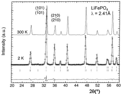
Figure 8. Observed (circles) versus calculated (continuous line) neutron powder diffraction patterns of \( LiFePO_{4} \) (D20, \( \lambda = 2.41 \) Å) at 2 K. The positions of the Bragg reflections are represented by vertical bars (first row = nuclear, second row = magnetic). The difference (obs–calc) pattern is displayed at the bottom of the figure. The pattern recorded at 300 K (i.e., above the magnetic transition) is displayed for comparison.
accuracy of the refined magnetic moment may be lower than that indicated by the least-squares standard deviation. Another explanation may be found in a non-negligible orbital contribution to the magnetic moment of \( Fe^{2+} \) . This ion presents a high-spin \( d^{6} \) configuration (weak crystal field), that is, four electrons on the three \( d_{xy} \) , \( d_{xz} \) , and \( d_{yz} \) ( \( t_{2g} \) ) orbitals, three of them being up and the fourth down, and one electron (spin up) on each \( e_{g} \) orbital ( \( d_{x^{2}-y^{2}} \) and \( d_{z^{2}} \) ). This configuration corresponds to S = 2, L = 2, noted \( {}^{5}D \) . As the angular moment is not equal to 0, \( Fe^{2+} \) may have a relatively strong spin–orbit coupling contributing to anisotropy and a non-quenched angular momentum that contributes to the magnetic moment. This may be the reason why the observed magnetic moment for \( Fe^{2+} \) , 4.19(5) \( \mu_{B} \) , is higher than what is expected on the basis of the spin-only value ( \( 4\mu_{B} \) ). An orbital momentum contribution to the experimental value of the magnetic moment has also been observed in \( Co^{2+} \) phosphates such as \( CoFePO_{5} \) . \( ^{22} \) Note that the magnetic structure we obtained is in perfect agreement with the structure determined by Santoro and Newman. \( ^{11} \) The final global refinement is shown in Figure 8 and a schematic of the corresponding magnetic structure is shown in Figure 9. The magnetic moments of \( Fe^{2+} \) atoms within the unit cell are indicated in Table 1, together with unit cell and atomic positions.
Magnetic Structure of \( FePO_{4} \) ( \( Fe^{3+} \) ). The same procedure was followed to solve the magnetic structure of \( FePO_{4} \) and over all the possibilities determined by symmetry analysis, the collinear solution \( A^{X} = (+ - - +) \) (antiferromagnetic ordering along [100]) gives the best agreement between observed and calculated patterns with a moment of 3.99(4) \( \mu_{B} \) . However, this solution underestimates the intensity of the (001) reflection (at \( 2\theta = 29.4^{\circ} \) , marked by an arrow in Figure 10). If we

Figure 9. Representation of the magnetic structure for \( LiFePO_{4} \) . Arrows indicate the magnetic moments on the iron atoms (along the b axis).

Figure 10. Observed (circles) versus calculated (continuous line) neutron powder diffraction patterns of $ FePO_{4} \( (D20, \lambda = 2.41 \AA) at 2 K. The positions of the Bragg reflections are represented by vertical bars (first Row = nuclear, second Row = magnetic). The difference (obs—calc) pattern is displayed at the bottom of the figure. The pattern recorded at 300 K i.e., above the magnetic transition) is displayed for comparison. The arrow indicates the (001) reflection that accounts for the \) G^{Y} = (+ - + -) \( component. consider a small component along the y-axis, with a spin sequence \( G^{Y} = (+ - + -) \) , the refinement is much improved. Introducing this component along y corresponds to a mixture of representations: \( \Gamma_{2}(A^{X} = S_{1}^{X} - S_{2}^{X} - S_{3}^{X} + S_{4}^{X}) + \Gamma_{1}(G^{Y} = S_{1}^{Y} - S_{2}^{Y} + S_{3}^{Y} - S_{4}^{Y}) \) .
Usually magnetic structures follow only one representation, and our particular case deserves a special comment. In \( FePO_{4} \) , iron is in the +3 oxidation state, with a spin configuration \( d^{5} \) . \( Fe^{3+} \) is a high-spin ion; that is, there is one spin (up) on each of the five orbitals ( \( d_{xy} \) , \( d_{xz} \) , \( d_{yz} \) , \( d_{x2-y2} \) , \( d_{z2} \) ), according to Hund's rule. This configuration corresponds to \( S = ^{5}/_{2} \) and L = 0, noted \( {}^{6}S \) . Contrary to \( Fe^{2+} \) , \( Fe^{3+} \) is a highly isotropic ion, and this may explain why we observe a mixture of representations. \( ^{22} \) We will see below that this is not the case. The obtained value for \( Fe^{3+} \) of 4.15(3) \( \mu_{B} \) (4.05(2) \( \mu_{B} \) along x and 0.90(6) \( \mu_{B} \) along y) is lower than the theoretical value of 5 \( \mu_{B} \) expected for \( Fe^{3+} \) (electronic configuration \( 3d^{5} \) , \( t_{2g}^{3} \) \( e_{g}^{2} \) ). Note that the value of the moment is determined with a much better accuracy.
Table 4. Comparison of the Different Magnetic Structures Observed in Olivines with Magnetic Ion on the M2 Site (4c) Only; A Corresponds to a Spin Sequence (+ - - +), G (+ - + -)
| olivine formula | magnetic atom | electronic configuration | magnetic structure | \( T_{\mathrm{N}} \) (K) | reference |
| LiMnPO4 | Mn2+ | 3d5 | A along a | 35 | 10 |
| FePO4 | Fe3+ | 3d5 | A along a + G along b | 125 | this work |
| LiFePO4 | Fe2+ | 3d6 | A along b | 50 | 11 |
| LiCoPO4 | Co2+ | 3d7 | A along b | 52 | this work |
| LiNiPO4 | Ni2+ | 3d8 | A along c | 23 | 8 |

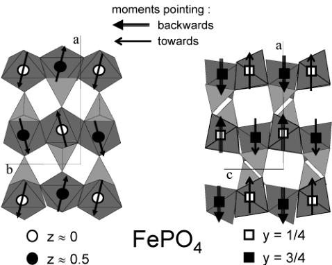
Figure 11. Representation of the magnetic structure for \( FePO_{4} \) . Arrows indicate the magnetic moments on the iron atoms (mainly along the a axis).
than that for \( LiFePO_{4} \) , as there are magnetic reflections having no nuclear contribution (e.g., (101)). The final refinement is shown in Figure 10, and the corresponding magnetic structure is shown in Figure 11. It is interesting to note that the magnetic structure is not collinear due to the y component of the magnetic moment, the sequence of which \( (G^{\mathrm{Y}}) \) is different from the component in the x direction \( (A^{\mathrm{X}}) \) : the magnetic moments of FeI and Fe2 are parallel to each other, as well as those of Fe3 and Fe4, but the directions of the FeI and Fe3 magnetic moments form an angle of \( 25^{\circ} \) (defined as \( 2\tan(M^{\mathrm{Y}}/M^{\mathrm{X}}) \) ). The magnetic moments of Fe atoms within the unit cell are indicated in Table 3, together with unit cell and atomic positions.
Comparison with \( LiMnPO_{4} \) , \( LiCoPO_{4} \) , and \( LiNiPO_{4} \) . It is interesting to compare the magnetic structure of \( FePO_{4} \) with \( LiMnPO_{4} \) , as \( Fe^{3+} \) (in \( FePO_{4} \) ) and \( Mn^{2+} \) (in \( LiMnPO_{4} \) ) present the same spin configuration \( 3d^{5} \) (both isotropic ions). \( LiMnPO_{4} \) was studied in the early 1960s. \( ^{10,11} \) The Néel temperature of \( LiMnPO_{4} \) is 35 K, much lower than the value we observe for \( FePO_{4} \) ( \( T_{N} = 125 \) K). The magnetic structure of \( LiMnPO_{4} \) has been found collinear along [100], with a spin sequence \( A^{X} \) , but no contribution along [010] was observed. The magnetic structures of \( LiCoPO_{4} \) and \( LiNiPO_{4} \) are collinear as well, \( ^{8} \) with a spin mode of A-type, but they differ in the spin direction. \( LiCoPO_{4} \) (highly anisotropic ion \( Co^{2+} \) ) has its magnetic moments along [010], exactly like the anisotropic \( LiFePO_{4} \) . The \( LiNiPO_{4} \) (isotropic \( Ni^{2+} \) ) magnetic structure is along [001]. The different magnetic structures observed, with the corresponding Néel temperatures, are reported in Table 4. Analysis and Discussion of the Magnetic Structure. Magnetic Phase Diagram. When lithium is extracted electrochemically or chemically from \( LiFePO_{4} \) to \( FePO_{4} \) , iron is oxidized from +2 to +3 and we found the following: (i) the Néel temperature was increased from 52 to 125 K; (ii) the sequence of the main spin component on the iron atoms for both compounds is the same (+ - - +), and (iii) the orientation of the magnetic moments are rotated by \( \pi/2 \) when lithium is extracted, from a collinear solution along the b-axis in \( LiFePO_{4} \) to a noncollinear solution mainly along the a-axis (plus a minor component along the b axis) in \( FePO_{4} \) .
The analysis of the diffraction patterns as a function of temperature shows that there is no change in the spin configuration in the whole range of the ordered state. We closely examined the relative strengths of the different exchange interactions within this crystal structure type to obtain the observed magnetic structure as the ground state, using the two programs, SIMBO and ENERMAG, which are shortly described in ref 23. Our analysis has neglected the anisotropy that may play a role in \( LiFePO_{4} \) . We followed the same procedure as we used for other iron phosphates. \( ^{[24,25]} \) An analysis of the exchange paths in both compounds leads to three different isotropic exchange interactions ( \( J_{i}, i = 1, 2, 3 \) ), numbered in ascending order of distances between magnetic atoms in \( FePO_{4} \) , all of them being of super-super exchange type except \( J_{1} \) , which is of super exchange type (only one oxygen involved in the path). Note that while the \( FePO_{4} \) framework and the space group are unchanged upon extraction of lithium from \( LiFePO_{4} \) to \( FePO_{4} \), the distances and angles characterizing the exchange paths are slightly different in both compounds.
Four atoms, labeled FeI, Fe2, Fe3, and Fe4, have to be taken into account in the structure, the second, third, and fourth being obtained from the first one by the symmetry operations of position 4c.
(a) The exchange integral \( J_{1} \) related to the shortest path (Fe–Fe at 3.8 Å) is the only one of super exchange type: it connects two irons atoms (FeI and Fe2, or Fe3 and Fe4) whose \( FeO_{6} \) octahedron shares a common corner O(3) (Figure 12). If we look at the structure as a stacking of \( TeOc_{2} \) planes along c, \( J_{1} \) is an interlayer interaction.
(b) The exchange integrals \( J_{2} \) and \( J_{3} \) connect iron atoms in a same (a, b) \( TeOc_{2} \) layer, as can be seen from Figure 12; \( J_{2} \) and \( J_{3} \) are of super-super exchange type.

Figure 12. Representation of the three exchange paths between the iron atoms that have to be considered in LiFePO_{4} and FePO_{4}. J_{1} ("interlayer") is of super exchange type, whereas J_{2} and J_{3} ("intralayer") are of super-super exchange type (two oxygen atoms involved in the path).

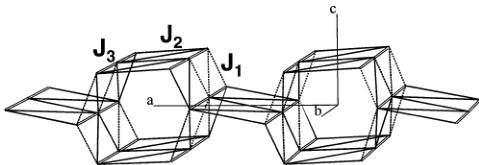
Figure 13. Topology of LiFePO_{4} and FePO_{4}: only exchange paths J_{1}, J_{2}, and J_{3} (connecting iron atoms) are represented.
Exchange paths corresponding to the integrals \( J_{1}, J_{2} \) , and \( J_{3} \) are represented in Figure 13. It is worth noting that the topology is complex and eventually subject to frustration: in a \( TeOc_{2} \) layer, iron atoms (connected via \( J_{2} \) and \( J_{3} \) ) form edge-sharing triangles, which are connected in chains running along b. We have calculated the phase diagram for the topology of this structural type and we can place on it the region (relative strengths and signs of the exchange interactions) corresponding to the observed magnetic structure as the ground state. We will use then the method discussed in refs 26–29 to evaluate the conditions satisfied by the exchange integrals in order to have the propagation vector \( \mathbf{k} = (0,0,0) \) and the observed antiferromagnetic spin arrangement \( (+ - - +) \) as ground state. We varied the values of all the exchange interactions \( J_{i} \) (i = 1, 2, 3) in the interval [-100, 100]. Only relative values are important for our purposes. The k-vectors were varied inside the Brillouin zone and in special points. An auxiliary program takes the output of ENERMAG \( ^{23} \) and plots a high-dimensional phase diagram using the exchange interactions as Cartesian axes. The different regions correspond to different magnetic structures. An analysis of the diagrams gives us immediately the conditions that the exchange integrals have to satisfy to give, as the first ordered state, the observed magnetic structure.
In LiFePO_{4} and FePO_{4}, the observed structure is k = (0,0,0) with a spin arrangement following the se-

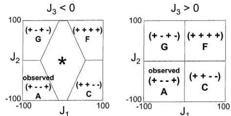
Figure 14. Magnetic phase diagrams for LiFePO_{4} and FePO_{4} considering three exchange integrals J_{1}, J_{2}, and J_{3}. The different spin sequences (all with k = (000)) are indicated on the figure, and the star (*) indicates incommensurate or disordered structures.
sequence: \( (+ - - +) \) (moments along [010] for LiFePO_{4}, and mainly along [100] for FePO_{4}). This structure can be obtained by considering the three exchange paths \( J_{1} \) , \( J_{2} \) , and \( J_{3} \) . The conditions to be satisfied by the exchange integrals to observe the sequence \( (+ - - +) \) are rather simple, as can be observed in Figure 14:
\[ for J_{3}<0:\ 2J_{1}+J_{2}<4J_{3} \]
\[ for J_{3}>0:\ J_{1}<0and J_{2}<0 \]
For \( J_{3} < 0 \) , the central domain (marked by *) corresponds to incommensurate or disordered structures. This domain is less and less important as \( J_{3} \) increases. \( J_{1} \) and \( J_{2} \) are of special importance, and they should both be negative to obtain the experimental magnetic structure as a ground state. \( J_{3} \) can be either positive or negative, provided the above conditions are fulfilled. However, \( (+ - - +) \) is observed as the ground state more “easily” if \( J_{3} > 0 \) .
Goodenough–Kanamori rules for super and supersuper exchange between two \( Fe^{3+} \) ( \( d^{5}-d^{5} \) at \( 180^{\circ} \) ) or two \( Fe^{2+} \) ( \( d^{6}-d^{6} \) at \( 180^{\circ} \) ) indicate that all these interactions should be antiferromagnetic, \( ^{30,31} \) the latter weaker than the former. This explains why \( T_{N} \) is much higher in \( FePO_{4} \) than in \( LiFePO_{4} \) . According to the Goodenough–Kanamori rules, the three exchange interactions \( J_{1} \) (super exchange) and \( J_{2} \) and \( J_{3} \) (super-super exchange) should be negative, that is, fulfill \( 2J_{1} + J_{2} < 4J_{3} \) . \( FePO_{4} \) is the only olivine compound (with the magnetic atom on the M2 site) for which the magnetic structure is noncollinear and corresponds to a mixture of representations \( (A^{X} + G^{Y}) \) . The reason we observe this noncollinear structure is still unclear. A mixture of representations occurs usually when both representations belong to the same exchange multiplet and give rise, in most cases, to a collinear (single-mode) magnetic structure. This is not the present case. Another reason may be the frustration present for \( J_{3} < 0 \) , and the degeneracy of the A and G modes for \( J_{2} \) are very small compared to the other exchange interactions. One could think as well at the Dzyaloshinky–Moriya interaction \( \mathbf{D}^{*}(\mathbf{S}_{i} \times \mathbf{S}_{j}) \) , which could induce a tilt of the magnetic moments similar to what is observed. Calculations and comple-
mentary experiments are in progress to explain this peculiar behavior of \( FePO_{4} \) .
Conclusion
The magnetic structures of \( LiFe^{II}PO_{4} \) and \( Fe^{III}PO_{4} \) have been solved from temperature-controlled neutron diffraction data. Differences in the Néel temperatures and reorientation of magnetic moments can be explained by the strong anisotropy of \( Fe^{2+} \) in \( LiFePO_{4} \) , whereas the isotropy of \( Fe^{3+} \) in \( FePO_{4} \) may explain why the structure is noncollinear. An analysis of the magnetic topology has been made, and numerical phase diagrams have allowed us to establish the relative stability regions of collinear magnetic structures for different values of the exchange interactions.
Acknowledgment. The authors wish to thank S. Gwizdala, C. Wurm, and E. Baudrin for fruitful discussions.
CM0300462
 p2_0.jpg
 p2_1.jpg
 p2_2.jpg
 p3_0.jpg
 p3_1.jpg
 p4_0.jpg
 p5_0.jpg
 p5_1.jpg
 p5_2.jpg
 p6_0.jpg
 p6_1.jpg
 p6_2.jpg
 p7_0.jpg
 p8_0.jpg
 p8_1.jpg
 p8_2.jpg