| Transition Temperature | 691.8 K |
|---|---|
| Experiment Temperature | 293 K |
| Propagation Vector | k1 (0, 0, 0) |
| Parent Space Group | Ima2 (#46) |
| Magnetic Space Group | Im'a'2 (#46.245) |
| Magnetic Point Group | m'm'2 (7.4.23) |
| Lattice Parameters | 5.66850 15.58230 5.52650 90.00 90.00 90.00 |
|---|---|
| DOI | 10.1006/jssc.2000.8998 |
| Reference | M. Schmidt, S. J. Campbell, Journal of Solid State Chemistry (2001) 156 292 - 304 |
| Label | Element | Mx | My | Mz | |M| |
|---|---|---|---|---|---|
| Fe1 | Fe | 0.0 | 0.0 | 3.92 | 3.92 |
| Fe2 | Fe | 0.0 | 0.0 | -3.92 | 3.92 |
Crystal and Magnetic Structures of Sr_{2}Fe_{2}O_{5} at Elevated Temperature
M. Schmidt \( ^{1} \)
Department of Applied Mathematics and Department of Electronic Materials Engineering, Research School of Physical Sciences and Engineering, The Australian National University, Canberra ACT 0200, Australia E-mail: marek.schmidt@ifmpan.poznan.pl.
and
S. J. Campbell
School of Physics, University College, The University of New South Wales, Australian Defence Force Academy, Canberra ACT 2600, Australia
Received June 19, 2000; in revised form September 14, 2000; accepted October 6, 2000; published online January 3, 2001
The evolution of crystal and magnetic structures of \( Sr_{2}Fe_{2}O_{5} \) with temperature was studied using neutron powder diffraction. The measurements were made in the temperature range from room temperature up to 1223.15 K and the patterns were analyzed using the Rietveld method. The oxide undergoes two phase transitions: (i) from the antiferromagnetic to the paramagnetic state and (ii) from the orthorhombic to the cubic structure. We discuss the changes of structural parameters with temperature and propose a new structural model for the cubic phase. The diffraction patterns were refined using \( I\hbar^{2}m^{2} \) , \( Ibm^{2} \) , and \( Fm^{3}c \) symmetry groups in the antiferromagnetic, the paramagnetic and the cubic state, respectively, with Z=4. © 2001 Academic Press
Key Words: \( Sr_{2}Fe_{2}O_{5} \) ; \( SrFeO_{x} \) ; strontium ferrite; oxygen conductor; antiferromagnet; Néel point; phase transition; crystal structure; magnetic structure; neutron diffraction.
1. INTRODUCTION
The oxide \( Sr_{2}Fe_{2}O_{5} \) ( \( SrFeO_{x} \) ) belongs to the non-stoichiometric strontium ferrite system \( SrFeO_{x} \) ( \( 2.5 \leq x \leq 3.0 \) ). The compound itself is a mixed oxygen conductor and investigation of its properties is important not only from the scientific point of view but also because of possible applications of the material or its derivatives (1). The material has been undergoing very intensive study for over four decades, but still lots of questions remain unanswered. In this paper we examine its magnetic and crystal structure at elevated temperature using neutron powder diffraction. The results of the experiments are analyzed using the Rietveld method. However, the method requires a model of ion distribution in the unit cell. Over the years of research there have been few attempts to solve its crystal structure at room temperature. Initially the oxide was assigned the Pcmn symmetry group based on the assumption that it is isomorphous with calcium ferrite \( Ca_{2}Fe_{2}O_{5} \) [2]. However, this choice was quickly dismissed by the results of magnetic structure investigation (3–5). Further study has shown that the oxide has a body-centered unit cell, and the observed systematic extinction pointed at two possible symmetry groups Icmn and Ibm2. The distinction between them was only possible on the basis of the goodness of fit between the observed and the calculated intensities. However, the oxide has a high melting point and, at the time, single crystals of the material were not available, so work was based on powder diffraction data. The refinement of the neutron powder pattern by Greaves et al. gave a better fit for the Icmn group (6). But, the authors acknowledged a possibility of a short-range Ibm2 order in the material. A subsequent single-crystal X-ray diffraction experiment proved the material has Ibm2 symmetry, and the better fit in the powder experiment was caused by stacking faults in the octahedron and tetrahedron layers along the orthorhombic b axis (7).
The behavior of the oxide at elevated temperature causes even more controversy, and published observations often contradict each other. It is an indisputable fact that the oxide undergoes two phase transitions between room temperature and 1223.15 K. The first one occurs around 673.15 K, and from the magnetic susceptibility measurements it is known to be the Néel point of the material (8, 9). The second one is a transformation from the orthorhombic to a cubic structure. However, there are two interpretations of this phase. The first one assumes that the oxide has a perovskite unit cell with disordered oxygen sites. This choice of unit cell was based on the belief that the structure is similar to the fully oxidized form \( SrFeO_{3} \) . This model was
challenged by Grenier et al. (9), whose group proposed a microdomain structure model based on the behavior of brownmillerite compounds doped with transition metals or lanthanides. The transition was reported within the temperature range 973.15–1123.15 K depending on the oxygen partial pressure in the atmosphere, which slightly alters the composition of the material (9–12). Published variations of lattice constants with temperature differ among the authors. Shin et al. (10) reported an increase of all three lattice constants up to the Néel point, then a decrease of one of them and continuous transformation to the cubic form. On the other hand, Takeda et al. (11) communicated a steady increase of all lattice parameters with temperature and the transition to the cubic structure with a substantial change in the unit cell volume. Grenier et al. (9) observed a two-phase mixture of the orthorhombic and a tetragonal phase between the Néel point and the temperature of transition to the cubic form.
The high-temperature form so far has only been studied using X-ray diffraction and the reports are confusing. We used different scattering methods to alleviate problems caused by the X-ray technique. Neutron diffraction was chosen to avoid problems caused by high-temperature X-ray cameras equipped with strip heaters. A large diffractometer furnace and a bulk sample used for the experiments eliminated the danger of big temperature gradients and the influence of surface phenomena such as surface oxidation or reaction with the heater. The experiments can give new insight into the material since the scattering mechanism is different from X-rays. Neutron scattering lengths of oxygen, iron, and strontium have comparable values, and the measurements are almost equally sensitive to all three elements. Their independence on the scattering angle allows us to extract the information even from high angle reflections. On the down side, the collected patterns suffer from the low resolution of the instrument, a common phenomenon among high-intensity constant-wavelength neutron diffractometers.
2. EXPERIMENTAL
The strontium ferrite \( (\mathrm{Sr}_{2}\mathrm{Fe}_{2}\mathrm{O}_{5}, \mathrm{F.W.} 366.93 \mathrm{~g/mol}) \) was prepared from dried hematite \( (\mathrm{Fe}_{2}\mathrm{O}_{3}, 99.9\% \text{ purity from Electronic Space Product International}) \) and strontium carbonate \( (\mathrm{SrCO}_{3}, 99.9 + \% \text{ purity from Aldrich}) \) combined in the molar ratio 1:2, respectively. The mixture was ball-milled for 12 h and then fired on an alumina combustion boat at 1373.15 K in air for a total of 55 h. During the procedure the sinter was ground and analyzed for traces of transient phases using X-ray powder diffraction. The annealing was finished upon the disappearance of the impurities. The material prepared this way usually has the oxygen stoichiometry x around 2.8. The oxide was again ground using a mortar and pestle and pressed into pellets under a pressure of 98 MPa. The pellets were reduced to \( Sr_{2}Fe_{2}O_{5} \) ( \( SrFeO_{2.5} \) ) by annealing at 1473.15 K in a flow of ultrahigh-purity argon (1.5 l/min, \( p_{O_{2}} < 1 \) ppm) for 8 h and cooled down in the inert atmosphere. The sintering yielded dense oxide cylinders 15 mm in diameter. The final product in powder form was brown, and its X-ray examination did not show any impurities or line broadening due to small crystal size. The Néel point and the temperature of the second phase transition were estimated using a differential scanning calorimeter (Shimadzu DSC-50) and a differential thermal analyzer (Shimadzu DTA-50), respectively, by heating the sample at a constant rate of 20 K/min in argon. Since the magnetic transition is of the second order, the peak of heat capacity at 668.15 K was taken as the temperature of transition. In the case of the second transformation the peak did not have the sharp onset characteristic for the first-order transformation. The slope of the DTA curve started slowly changing around 1073.15 K and the transformation was completed around 1173.15 K, so the value corresponding to the peak of the heat capacity at 1140.15 K was again taken as the temperature of transformation.
Neutron diffraction patterns were collected using the Medium Resolution Powder Diffractometer (MRPD) at the Australian Nuclear Science and Technology Organisation in Lucas Heights (New South Wales). The diffractometer operates in the Debye–Scherrer geometry, and its instrumental profile width (FWHM) ranges between \( 0.4^{\circ} \) and \( 0.8^{\circ} \) (13). The data were collected in the angular range of \( 5-138^{\circ} \) with \( 0.1^{\circ} \) increments using a bank of 32 detectors. To avoid the influence of neutron intensity fluctuations, the detectors, at every angle, counted until the beam monitor registered a certain number of a neutrons. The diffraction experiments were made using a neutron wavelength of \( 1.6672 \AA \) , and the Rietveld refinement was carried out using the GSAS program (14). The diffraction peaks were represented using the asymmetric Gauss function (15–17), and the dependence of the profile width on the diffraction angle was modeled using the Caglioti formula (18). The only refined profile parameters were U, V, and W. The asymmetry parameter was kept constant, and \( F_{1} \) , \( F_{2} \) coefficients were set to zero. For the experiments the diffractometer was equipped with a furnace, and to protect the material against oxidation the pellets were placed in a silica tube in a flow of ultra-high-purity argon. The patterns were collected in the temperature range from room (293.15 K) to 1223.15 K. Before each acquisition the sample was kept at a given temperature for at least 15 min. Unfortunately, the furnace introduced a small peak centered about \( 27.4^{\circ} \) , and for this reason the region from \( 26.5^{\circ} \) to \( 28.5^{\circ} \) was excluded from the refinement. The furnace peak overlaps with the (121) reflection of the orthorhombic phase. Apart from the peak the furnace and the silica tube are sources of diffuse background, which combined with the sample contribution gave a complicated curve. The background was not very intense compared to the diffraction peaks and it was simulated using the linear
interpolation function (23 coefficients). Attempts to refine it using polynomials, Fourier series, or a real space correlation function did not give satisfactory results.
3. RESULTS AND DISCUSSION
Analysis of the calorimetric information suggests that the entire temperature range in question can be divided into three parts. In the divisions the sample exists as: (i) the orthorhombic antiferromagnet, (ii) the paramagnetic phase, and (iii) the cubic phase, respectively. The diffraction patterns revealed that the oxide does not change its crystal structure upon the transformation from the magnetically ordered to the paramagnetic state and the orthorhombic structure transforms into the cubic as previously observed. However, the neutron diffraction uncovered the existence of the fourth region in the vicinity of the second-phase transition. In this range, the material exists as a mixture of the orthorhombic and the cubic phases. It is difficult at this stage to establish the exact temperature range, but abnormal values of the lattice parameters suggest that it spans over the temperature domain of the DTA peak \( (1073.15 < T < 1173.15) \) . All data describing the crystal structure was extracted using the Rietveld method. But let us first discuss the changes in the lattice parameters without venturing into the details concerning the distribution of atoms in the unit cell. This information, in principle, can be obtained without the analysis of the cell content. The changes of the orthorhombic lattice constants with temperature

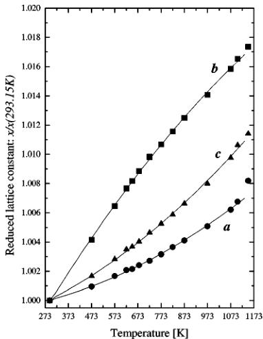
FIG. 1. Reduced orthorhombic lattice constants as functions of temperature. Lines are the results of fitting with parabolic functions.
TABLE 1
The Polynomial Coefficients Obtained by Fitting of the Orthorhombic Lattice Parameters
| Lattice parameter | \( \alpha_{0} \) | \( \alpha_{1} \) | \( \alpha_{2} \) |
| a | 5.6638(9) | 89(27) \( \times \) 10 \( ^{-7} \) | 2.7(2) \( \times \) 10 \( ^{-8} \) |
| b | 15.456(5) | 4.54(13) \( \times \) 10 \( ^{-4} \) | -9.9(9) \( \times \) 10 \( ^{-8} \) |
| c | 5.516(2) | 2.6(5) \( \times \) 10 \( ^{-5} \) | 3.17(33) \( \times \) 10 \( ^{-8} \) |
| V | 481.8(2) | 0.02044(26) | — |
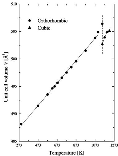
are presented in Fig. 1. It shows reduced values obtained by division of the constants by the room temperature value. This way all three parameters can be plotted in one picture and compared. The lattice expansion is anisotropic, and the variation of the lattice constants between room temperature and 1073.15 K can be satisfactory described using a parabolic equation: \( y(T) = \alpha_{2}T^{2} + \alpha_{1}T + \alpha_{0} \) . The results of fitting with the polynomials are presented in Table 1 and plotted in Fig. 1 as solid lines. The rate of expansion is different for all three directions, and the dilation along the b axis slows down with increasing temperature. The maximum expansion reaches 1.6% and is comparable with dilatation of metals such as nickel or copper in the same temperature range. Above 1073.15 K the lattice expands even faster. The unit cell volume V as a function of temperature is presented in Fig. 2. Surprisingly, the different rates of expansion of the cell edges yield a linear increase of the orthorhombic unit cell volume between room temperature

FIG. 2. The unit cell volume as a function of temperature.

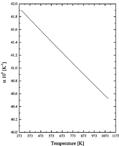
FIG. 3. The volume thermal expansion coefficient of the orthorhombic phase as a function of temperature.
and 1073.15 K. For this scope it is possible to calculate the volume thermal expansion coefficient \( \alpha \equiv \frac{\langle \delta V \rangle}{\langle T \rangle} p \) using the linear approximation. The result is shown in Fig. 3. Its value decreases with temperature, but above 1073.15 K it should increase again. However there are not enough points to calculate the derivative. The coefficient can be useful for thermodynamical calculations such as evaluation of the entropy changes \( \left(\frac{\delta S}{\delta p}\right)_{T} = V \alpha \) or to assess the oxide's mechanical compatibility with other materials at high temperatures. The volumes of the orthorhombic and subsequently the cubic cells have abnormal values in the temperature range corresponding to the second phase transition. Above it the cubic cell volume increases with temperature. It should be noted, however, that the volume before the transformation (at 1073.15 K) is almost equal to the volume of the cubic cell after the transition (at 1173.15 K).
3.1. The Orthorhombic Form
The refinement of the orthorhombic structure was carried out using the \( I b^{m}2 \) Shubnikov group to accommodate the magnetic reflections and the \( I b m2 \) symmetry group, below and above the Néel point, respectively, assuming isotropic thermal vibrations of atoms. This is of course a simplification, but in our opinion reliable values of the anisotropic thermal coefficients can only be found by analyzing larger data sets. The coordinates of atoms in the unit cell, varied during the refinement, are presented in Table 2, and all sites in the structure are fully occupied. The initial values for the refinement were taken from the single-crystal work of
TABLE 2
Coordinates of Atoms in the Orthorhombic Unit Cell Varied during the Refinement
| Atom | Wyckoff notation | x | y | z |
| Sr | 8c | r | r | r |
| Fe(1) | 4a | 0 | 0 | 0 |
| Fe(2) | 4b | r | 0.25 | r |
| O(1) | 8c | r | r | r |
| O(2) | 8c | r | r | r |
| O'(3) | 4b | r | 0.25 | r |
Note. Here, “r” indicates refined.
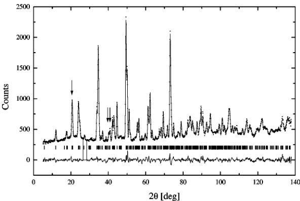
Harder and Müller-Buschbaum (7). The results are presented in Table 3 and Table 4 for the antiferromagnetic and the paramagnetic states, respectively. The examples of refined patterns are shown in Fig. 4. The picture contains patterns below and above the Néel point; its most conspicuous feature is the disappearance of the magnetic reflections. The reduced coordinates of atoms are similar to the result of the room-temperature single-crystal experiment and do not change significantly with temperature. The only difference is the z coordinate of O(2), virtually equal zero. Values of the thermal factors increase with temperature as expected, and the thermal parameters of iron Fe(2) and oxygen O(3) are abnormally high as previously reported (6). However, the difference becomes less significant as temperature increases. The distribution of atoms in the crystal structure is shown in Fig. 12. It contains a fragment of the crystal structure whose significance will be explained in the last section. We are referring to the figure now just to avoid plotting the same structure twice. Iron atoms have two different surroundings. The iron in site 4a is octahedrally coordinated, and the values of bond lengths and angles are presented in Table 5. Because oxygen O(1) does not lie in the same plane with iron Fe(1), the resulting octahedron is distorted. Also a non-zero x coordinate of oxygen O(2) causes the octahedron (Fe(1)–O(2) bond) to tilt in the ab plane. The tilt angle is decreasing with temperature from 7.4° at room temperature to 7° at 1073.15 K, and the neighboring rows of octahedrons along the c axis are tilted in the opposite direction. The lengths of Fe(1)–O(1) bonds remain essentially constant, and only the Fe(1)–O(2) bond visibly increases with temperature. Also, small changes in angles are noticeable. The tetrahedral surrounding of iron Fe(2) is created by oxygens O(2) and O(3). The values of obtuse angles and bonds are presented in Table 6. Oxygen atoms do not form an ideal tetrahedron. The lengths of both Fe(2)–O(2) bonds are equal and constant. Only one of Fe(2)–O(3) bonds and the O(2)–Fe(2)–O(2) angle are increasing with temperature. And just for the sake of completeness the bond lengths of the strontium polyhedron created by oxygens O(1), O(2), and O(3) are presented in Table 7.
TABLE 3
Refinement Results for the Antiferromagnetic Phase at Different Temperatures
| 293.15 K | 473.15 K | 573.15 K | 623.15 K | 648.15 K | 678.15 K | ||
| a(Å) | 5.66850(35) | 5.6739(4) | 5.6780(4) | 5.6803(4) | 5.6807(4) | 5.6822(4) | |
| b(Å) | 15.5823(8) | 15.6470(8) | 15.6830(9) | 15.7019(9) | 15.7096(9) | 15.7203(9) | |
| c(Å) | 5.52653(32) | 5.53580(33) | 5.5422(4) | 5.54587(35) | 5.5469(4) | 5.5488(4) | |
| V(ų) | 488.15(5) | 491.46(5) | 493.52(5) | 494.64(5) | 495.01(5) | 495.65(5) | |
| mz(μB) | 3.92(3) | 3.28(3) | 2.72(3) | 2.25(3) | 1.99(3) | 1.38(4) | |
| Sr | x | 0.0163(7) | 0.0152(7) | 0.0150(8) | 0.0148(8) | 0.0141(8) | 0.0152(8) |
| Sr | y | 0.10890(19) | 0.10930(21) | 0.10936(23) | 0.10989(22) | 0.10986(22) | 0.10993(22) |
| Sr | z | 0.4989(27) | 0.4995(24) | 0.5005(23) | 0.5011(23) | 0.5008(24) | 0.4985(23) |
| Sr | U | 0.64(9) | 0.95(9) | 0.97(10) | 1.18(10) | 1.19(10) | 1.18(10) |
| Fe(1) | U | 0.88(9) | 1.33(10) | 1.65(11) | 1.71(11) | 1.78(11) | 1.84(11) |
| Fe(2) | x | 0.9355(8) | 0.9359(8) | 0.9367(8) | 0.9367(8) | 0.9369(8) | 0.9382(8) |
| Fe(2) | z | 0.9833(24) | 0.9756(23) | 0.9715(24) | 0.9702(24) | 0.9700(24) | 0.9675(23) |
| Fe(2) | U | 2.49(13) | 2.55(15) | 2.48(15) | 2.46(15) | 2.57(16) | 2.24(15) |
| O(1) | x | 0.2574(24) | 0.2545(26) | 0.2510(29) | 0.2480(29) | 0.2438(25) | 0.2438(24) |
| O(1) | y | 0.99123(29) | 0.99158(31) | 0.99176(33) | 0.99185(32) | 0.99215(34) | 0.99181(33) |
| O(1) | z | 0.2537(35) | 0.2589(33) | 0.2586(35) | 0.2528(36) | 0.2513(35) | 0.2529(33) |
| O(1) | U | 0.09(12) | 0.45(13) | 0.6(13) | 0.79(11) | 0.96(12) | 0.75(12) |
| O(2) | x | 0.0500(8) | 0.0506(8) | 0.0500(9) | 0.0485(9) | 0.0486(9) | 0.0490(9) |
| O(2) | y | 0.14109(26) | 0.14127(28) | 0.14115(29) | 0.14126(29) | 0.14109(30) | 0.14119(30) |
| O(2) | z | 0.0010(36) | -0.0041(36) | -0.0029(35) | -0.0006(33) | -0.0060(36) | -0.0054(34) |
| O(2) | U | 1.03(11) | 1.64(12) | 1.84(13) | 2.18(13) | 2.23(13) | 2.39(13) |
| O(3) | x | 0.8568(15) | 0.8600(17) | 0.8586(17) | 0.8566(17) | 0.8579(17) | 0.8556(17) |
| O(3) | z | 0.6224(29) | 0.6236(30) | 0.6228(31) | 0.6205(30) | 0.6196(30) | 0.6208(29) |
| O(3) | U | 1.39(20) | 2.22(23) | 2.29(25) | 2.41(24) | 2.56(25) | 2.69(26) |
| Rwp(%) | 4.37 | 4.23 | 4.18 | 4.01 | 4.06 | 3.93 | |
| Rp(%) | 3.39 | 3.36 | 3.26 | 3.12 | 3.20 | 3.15 | |
| χ² | 5.670 | 3.515 | 3.427 | 3.145 | 3.221 | 3.023 |
Note. \( U = 100U_{iso} \)
3.2. The Magnetic Structure
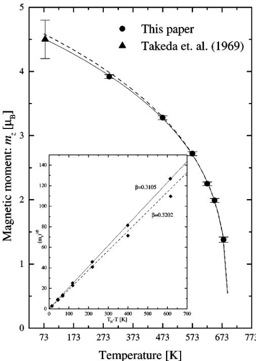
The primary aim of this paper is to describe the evolution of the crystal structure with temperature. However, neutron diffraction is sensitive to the magnetic order and this information had to be taken into consideration during the refinement. The investigation of magnetic structure is hampered by the fast decay of the magnetic form factor with scattering angle and the fact that we can only observe three reasonably strong magnetic reflections. Thorough study of this structure should employ longer neutron wavelengths which would separate the overlapping magnetic reflections. The magnetic peaks were generated simultaneously with the nuclear ones using the \( Ib'm'2 \) Shubnikov group derived from the \( Ibm'2 \) symmetry group, and the choice was made on the basis of the best fit to the experimental intensities. The group constrains magnetic moment of the octahedral iron Fe(1) along the c axis and allows the moment of tetrahedral iron Fe(2) to assume any direction in the ac plane. But, the tetrahedral moment was constrained along the c axis too, since any attempts to refine the component along the a axis led to a fast divergence of refinement. The resulting magnetic model is the same as that used in previous investigations of the structure at low temperatures (3, 6). However, the analysis of the magnetic structure at elevated temperatures can be cramped by decreasing the value of the antiferromagnetic coupling which manifests itself as the decaying magnetic moment. Weak magnetic reflections close to the ordering temperature can yield corrupted results, so the refinement was stabilized by an additional constraint: \( m_{z}(\mathrm{Fe}(2)) = -m_{z}(\mathrm{Fe}(1)) \) . It assures zero net magnetic moment of the structure and can be introduced since the magnetic susceptibility measurements (8, 9) and the magnetization measurements at room temperature, done by the authors using a vibrating sample magnetometer, did not shown any magnetic moment in the absence of the external field. The magnetic moment as a function of temperature is presented in Fig. 5; its magnitude decreases as temperature approaches the Néel point. However, the ordering temperature found using the calorimeter is underestimated, and the long-range magnetic order vanishes above it. Neutron measurements give the true value of the transition point since the method is sensitive to the magnetic structure and a calorimeter can pick up heat changes caused by other phenomena preceding the transition. The collected data does not allow us to establish
TABLE 4
Refinement Results for the Paramagnetic Phase at Different Temperatures
| 723.15 K | 773.15 K | 823.15 K | 873.15 K | 973.15 K | 1073.15 K | 1103.15 K | 1148.15 K \( ^{a} \) | ||
| a( \( \textup{\AA} \) ) | 5.6839(4) | 5.6864(4) | 5.6892(4) | 5.6918(4) | 5.6973(4) | 5.7037(4) | 5.7068(4) | 5.7149(5) | |
| b( \( \textup{\AA} \) ) | 15.7354(9) | 15.7488(9) | 15.7626(10) | 15.7769(9) | 15.8016(10) | 15.8292(10) | 15.8401(10) | 15.8528(13) | |
| c( \( \textup{\AA} \) ) | 5.5522(4) | 5.5556(4) | 5.5590(4) | 5.5632(4) | 5.5707(4) | 5.5805(4) | 5.5853(4) | 5.5896(5) | |
| V( \( \textup{\AA}^{3} \) ) | 496.58(5) | 497.53(6) | 498.51(6) | 499.57(6) | 501.51(6) | 503.84(6) | 504.89(6) | 506.41(7) | |
| Sr | x | 0.0137(8) | 0.0146(8) | 0.0147(8) | 0.0156(8) | 0.0143(9) | 0.0142(9) | 0.0133(9) | 0.0139(12) |
| Sr | y | 0.11004(22) | 0.10962(22) | 0.10985(22) | 0.11040(22) | 0.11075(24) | 0.11135(23) | 0.11152(24) | 0.11113(35) |
| Sr | z | 0.4985(23) | 0.5029(24) | 0.5021(26) | 0.5027(24) | 0.5038(25) | 0.5024(24) | 0.5037(26) | 0.5017(34) |
| Sr | U | 1.29(10) | 1.57(11) | 1.62(11) | 1.75(11) | 1.97(12) | 2.29(12) | 2.40(13) | 2.47(18) |
| Fe(1) | U | 1.99(11) | 2.23(11) | 2.21(11) | 2.53(12) | 2.70(13) | 3.14(13) | 3.26(14) | 3.14(20) |
| Fe(2) | x | 0.9376(8) | 0.9374(8) | 0.9368(9) | 0.9393(9) | 0.9396(9) | 0.9394(9) | 0.9396(9) | 0.9400(12) |
| Fe(2) | z | 0.9689(24) | 0.9748(25) | 0.9762(26) | 0.9707(25) | 0.9708(26) | 0.9684(24) | 0.9712(27) | 0.9690(33) |
| Fe(2) | U | 2.50(15) | 2.55(15) | 2.71(15) | 2.79(16) | 2.72(17) | 2.81(17) | 2.79(17) | 2.86(23) |
| O(1) | x | 0.2484(30) | 0.2569(26) | 0.2573(27) | 0.2417(23) | 0.2412(24) | 0.2380(21) | 0.2418(25) | 0.2439(39) |
| O(1) | y | 0.99219(34) | 0.99185(33) | 0.99176(35) | 0.99216(35) | 0.99230(38) | 0.99196(37) | 0.99241(39) | 0.9913(5) |
| O(1) | z | 0.2532(37) | 0.2543(36) | 0.2543(39) | 0.2486(34) | 0.2501(37) | 0.2486(35) | 0.2463(38) | 0.2546(6) |
| O(1) | U | 1.11(12) | 0.96(13) | 1.21(14) | 1.40(12) | 1.50(13) | 2.07(14) | 2.14(14) | 2.29(21) |
| O(2) | x | 0.0477(9) | 0.0487(9) | 0.0482(10) | 0.0482(10) | 0.0469(11) | 0.0474(11) | 0.0465(11) | 0.0486(15) |
| O(2) | y | 0.14121(30) | 0.14178(29) | 0.14146(31) | 0.14165(30) | 0.14161(33) | 0.14140(33) | 0.14103(34) | 0.1428(5) |
| O(2) | z | -0.0031(35) | 0.0029(32) | 0.0003(36) | -0.0017(33) | -0.0034(37) | -0.0037(35) | 0.0030(36) | -0.005(5) |
| O(2) | U | 2.61(13) | 2.45(14) | 2.66(14) | 2.69(14) | 3.25(16) | 3.71(16) | 4.04(18) | 4.23(24) |
| O(3) | x | 0.8577(17) | 0.8595(18) | 0.8589(18) | 0.8571(17) | 0.8573(19) | 0.8544(18) | 0.8546(19) | 0.8581(27) |
| O(3) | z | 0.6210(31) | 0.6242(31) | 0.6254(33) | 0.6222(30) | 0.6241(32) | 0.6271(31) | 0.6333(34) | 0.623(5) |
| O(3) | U | 2.98(27) | 3.20(27) | 3.21(27) | 3.30(28) | 3.61(32) | 4.10(33) | 4.40(34) | 5.22(50) |
| R \( _{\textup{wp}} \) (%) | 3.76 | 3.82 | 3.81 | 3.67 | 3.80 | 3.56 | 3.51 | 2.97 | |
| R \( _{\textup{p}} \) (%) | 2.95 | 2.99 | 3.00 | 2.88 | 2.95 | 2.81 | 2.84 | 2.40 | |
| \( \chi^{2} \) | 2.778 | 2.867 | 2.864 | 2.654 | 2.861 | 2.551 | 2.497 | 1.794 |
Note. \( U = 100U_{iso} \)
\( ^{a} \) two phase pattern.
the temperature by a simple extrapolation. However, the molecular-field theory shows that in the vicinity of the critical temperature \( T_{N} \) the moment should tend to zero with temperature like \( (T_{N}-T)^{\beta} \) as \( T\to T_{N} \) , where \( \beta=\frac{1}{2} \) . More sophisticated theories and other experimental results indicate that \( \beta\simeq\frac{1}{3} \) (19), so the magnetic moment close to the Néel point should vary according to the equation
\[ m_{z}=A(T_{N}-T)^{\beta}, \quad [1] \]
where A is a constant. Values of the critical temperature \( T_{N} \) and the critical index \( \beta \) were found by a nonlinear fitting of the equation:
\[ \ln m_{z}=\beta\ln(T_{N}-T)+\ln A. \quad [2] \]
The results differ from each other depending on how many points were used for the calculations. Fitting all six points yields the result shown as the solid line in Fig. 5. Apart from the data collected by the authors it also contains the magnetic moment at 77 K found by Takeda et al. (3). But this point was not used for the calculations and is there for the reference only. The same curve was also drawn as a straight line in the inset by recalculating the data using the equation
\[ (m_{z})^{1/\beta}=B(T_{N}-T), \quad [3] \]
where B is a constant. It gives almost perfect fit and \( \beta = 0.3105 \) , \( T_{N} = 691.8 \) K. However, this result is not physical since the approximation works only close to the critical temperature. At low temperatures the derivative \( \frac{dm_{z}}{dT} \) should approach zero as temperature approaches 0 K. In other words, the moment should saturate and points at lower temperatures ought to lie below the calculated curve. The values of the critical temperature and the critical index, obtained from the six-point fit, should be treated as the lower limit of the real ones. From the physical point of view the best solution is obtained by fitting the curve to four points closest to the transition temperature. It yields \( \beta = 0.3202 \) , \( T_{N} = 692.8 \) K and is presented in Fig. 5 as the dashed line. The new value of the Néel point is very close to the number obtained by the six-point fit, and the low temperature points lie under the curve. More precise determination of the ordering temperature and the critical index require collection of many more experimental points in the direct proximity of the transition point, and the values just


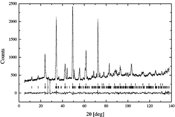
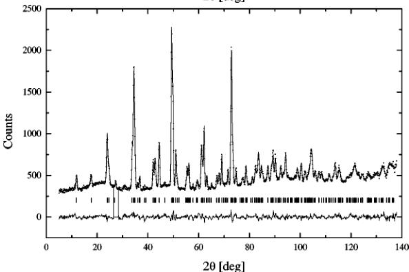
FIG. 4. Examples of refined orthorhombic patterns below the Néel point at 573.15 K (top) and above at 773.15 K (bottom). The arrows mark the positions of the three strongest magnetic reflections.
presented should be seen as the best results that can be obtained from a fairly small data set.
The long-range magnetic order vanishes at 692.8 K; however, some residual short-range ordering remains and manifests itself as a small diffused peak around \( 30.9^{\circ} \) . It persists until the structure changes over into the cubic.
3.3. The Cubic Phase
The material transformed into the cubic form above 1148.15 K. Previously this phase was thought to have the cubic perovskite structure with disordered oxygen sites (10, 11). Shin et al. reported the lattice constant of 3.982 Å at 1173.15 K and Pm3m symmetry group (10, 20). However, if we assume that the cell contains only one chemical formula (molecule) of the oxide, this choice of unit cell gives unreasonably high density \( \varrho = 9.65 \, g/cm^3 \) . The calculated value is almost twice the density of the material at room temperature. Moreover, it is impossible to accommodate a nine-atom molecule in the cell and still get the perovskite structure. The wrong choice was biased by the fact that the fully oxidized \( SrFeO_3 \) phase forms such a structure and has similar lattice constant (10). High calculated density indicates that the perovskite cell, obtained by direct indexing of the patterns, is too small to describe the compound. The problem was solved by doubling the primitive constant. The resulting cell has eight times greater volume, and if we assume that it contains four chemical formulas (Z = 4) it yields sensible density. As a result the primitive Miller indexes (hkl) are multiplied by a factor of two and give a new set of conditions for the observed reflections: hkl: \( h + k, k + l, l + h = 2n \) ; hhl: \( h, l = 2n \) ; 0kl: \( k, l = 2n \) . The
TABLE 5
Octahedral Bond Lengths (in Angstroms) and Angles (in Degrees) as a Function of Temperature
| T (K) | Fe(1)-O(1) | Fe(1)-O(1) | O(1)-Fe(1)-O(1) | O(1)-Fe(1)-O(O1) | Fe(1)-O(2),[2] | O(1)-Fe(1)-O(2) | O(1)-Fe(1)-O(2) |
| 293.15 | 2.028(17) | 1.94(17) | 92.5(9) | 88.301(27) | 2.217(4) | 88.3(8) | 90.9(6) |
| 473.15 | 2.039(18) | 1.933(18) | 90.7(9) | 88.316(33) | 2.229(4) | 88.3(8) | 92.7(6) |
| 573.15 | 2.025(20) | 1.951(20) | 89.9(9) | 88.344(33) | 2.232(5) | 88.3(8) | 93.4(6) |
| 623.15 | 1.991(21) | 1.986(20) | 90.5(9) | 88.395(22) | 2.235(5) | 88.4(8) | 92.7(5) |
| 648.15 | 1.969(19) | 2.009(19) | 89.9(9) | 88.436(25) | 2.234(5) | 88.4(9) | 93.3(5) |
| 678.15 | 1.976(18) | 2.004(18) | 89.5(8) | 88.419(27) | 2.237(5) | 88.4(8) | 93.7(5) |
| 723.15 | 1.996(21) | 1.984(21) | 90.5(9) | 88.444(23) | 2.239(5) | 88.4(9) | 92.7(5) |
| 773.15 | 2.037(18) | 1.946(18) | 92.1(10) | 88.446(29) | 2.25(5) | 88.4(8) | 91.0(6) |
| 823.15 | 2.039(19) | 1.947(19) | 92.3(10) | 88.453(31) | 2.247(5) | 88.5(9) | 90.8(7) |
| 873.15 | 1.954(18) | 2.033(18) | 89.9(8) | 88.506(26) | 2.252(5) | 88.5(8) | 93.1(5) |
| 973.15 | 1.961(19) | 2.031(19) | 89.4(9) | 88.541(29) | 2.254(5) | 88.5(9) | 93.5(5) |
| 1073.15 | 1.945(18) | 2.053(18) | 89.0(8) | 88.587(31) | 2.255(5) | 88.6(8) | 93.8(5) |
| 1103.15 | 1.953(20) | 2.047(20) | 90.3(9) | 88.59(29) | 2.25(6) | 88.6(8) | 92.5(5) |
| 1148.15a | 1.996(30) | 2.011(30) | 89.1(13) | 88.47(4) | 2.28(8) | 88.5(12) | 93.9(8) |
Note. The figure in square brackets denotes the number of bonds when they have equal length.
\( ^{a} \) Two-phase pattern.
conditions are fulfilled by the \( Fm3c \) (226) symmetry group. The atoms were placed in the special positions of the group given in Table 8. The proposed cell consists of eight adjacent perovskite blocks. The iron ions are situated in the octahedral sites; however, statistically four of them have one oxygen missing. The positions of the atoms in the cell are fixed by the symmetry. Twenty oxygen ions, in this arrangement, are randomly distributed among 24 available sites. The refinement was carried out with fixed site occupancy. At the end of the process the occupancy factor for oxygen was refined. It led to the convergence; however, it did not significantly improve the fit and the refined occupancy value corresponded to approximately 19.66 oxygen atoms per unit cell. This implies that the oxide may contain a significant amount (8.5%) of iron in the \( 2+ \) oxidation state. The ferrite was tested for the presence of the ferrous ion using 0.1% water solution of o-phenanthroline (1,10-phenanthroline hydrate, \( C_{12}H_{8}N_{2}\cdotH_{2}O \) ). A small amount of the oxide was dissolved in hydrochloric acid, and a drop of the solution was quickly transferred onto a spot plate and mixed with a drop of the reagent. The test did not show the presence of the \( Fe^{2+} \) . The concentration limit for the test is 1 in 1,500,000 (21). So the oxygen occupancy was set back to the initial value of \( \frac{2}{24} \) and kept fixed. The only refined structural parameters were the
TABLE 6
Tetrahedral Bond Lengths (in Angstroms) and Angles (in Degrees) as a Function Of Temperature
| T (K) | Fe(2)-O(2),[2] | Fe(2)-O(3) | Fe(2)-O(3) | O(2)-Fe(2)-O(2) | O(2)-Fe(2)-O(3),[2] | O(3)-Fe(2)-O(3) |
| 293.15 | 1.820(5) | 2.044(13) | 1.827(10) | 137.7(4) | 107.5(4) | 102.3(4) |
| 473.15 | 1.825(5) | 1.995(13) | 1.868(10) | 137.6(4) | 107.1(4) | 103.6(4) |
| 573.15 | 1.830(5) | 1.983(13) | 1.875(11) | 137.8(5) | 106.2(4) | 103.6(4) |
| 623.15 | 1.829(5) | 1.992(13) | 1.863(10) | 138.0(5) | 105.72(34) | 103.4(4) |
| 648.15 | 1.830(5) | 1.995(13) | 1.869(10) | 138.5(5) | 106.2(4) | 103.3(4) |
| 678.15 | 1.829(5) | 1.980(13) | 1.874(10) | 138.5(5) | 105.6(4) | 103.3(4) |
| 723.15 | 1.829(5) | 1.985(13) | 1.879(10) | 138.7(5) | 105.52(35) | 103.5(4) |
| 773.15 | 1.825(5) | 1.998(14) | 1.881(11) | 138.1(5) | 105.87(34) | 103.4(4) |
| 823.15 | 1.829(5) | 2.000(14) | 1.875(11) | 138.5(5) | 106.2(4) | 104.3(4) |
| 873.15 | 1.825(5) | 1.995(13) | 1.886(10) | 139.0(5) | 105.4(4) | 103.0(4) |
| 973.15 | 1.824(6) | 1.988(14) | 139.7(6) | 105.3(4) | 103.1(4) | |
| 1073.15 | 1.833(6) | 1.965(14) | 1.895(11) | 139.4(6) | 104.9(4) | 103.6(4) |
| 1103.15 | 1.839(6) | 1.948(15) | 1.907(12) | 139.6(6) | 104.2(4) | 103.9(4) |
| 1148.15a | 1.816(9) | 1.988(21) | 1.910(16) | 138.9(8) | 105.6(6) | 103.2(6) |
Note. The figures in square brackets denote the number of bonds or angles when they have equal value.
\( ^{a} \) Two-phase pattern.
TABLE 7
Strontium Polyhedron Bond Lengths (in Angstroms) as a Function of Temperature
| T (K) | Sr-O(1) | Sr-O(1) | Sr-O(1) | Sr-O1) | Sr-O(2) | Sr-O(2) | Sr-O(2) | Sr-O3) |
| 293.15 | 2.658(14) | 2.584(15) | 2.644(13) | 2.563(14) | 2.804(21) | 2.826(21) | 2.509(5) | 2.473(7) |
| 473.15 | 2.648(13) | 2.571(14) | 2.676(12) | 2.596(13) | 2.840(20) | 2.800(21) | 2.514(6) | 2.469(7) |
| 573.15 | 2.645(14) | 2.568(15) | 2.686(13) | 2.609(14) | 2.841(19) | 2.804(20) | 2.520(6) | 2.472(7) |
| 623.15 | 2.662(14) | 2.584(15) | 2.683(13) | 2.607(14) | 2.832(18) | 2.813(19) | 2.529(6) | 2.467(7) |
| 648.15 | 2.653(14) | 2.575(14) | 2.691(13) | 2.618(13) | 2.861(19) | 2.786(19) | 2.532(6) | 2.463(7) |
| 678.15 | 2.644(13) | 2.565(14) | 2.705(12) | 2.632(12) | 2.845(18) | 2.803(19) | 2.524(6) | 2.476(7) |
| 723.15 | 2.660(14) | 2.581(15) | 2.696(13) | 2.619(14) | 2.834(19) | 2.817(20) | 2.541(6) | 2.470(7) |
| 773.15 | 2.691(15) | 2.616(16) | 2.661(13) | 2.580(14) | 2.830(19) | 2.830(19) | 2.534(6) | 2.474(8) |
| 823.15 | 2.696(16) | 2.619(17) | 2.666(14) | 2.583(15) | 2.840(20) | 2.820(21) | 2.536(6) | 2.477(8) |
| 873.15 | 2.671(13) | 2.600(13) | 2.694(12) | 2.630(13) | 2.855(18) | 2.807(18) | 2.532(6) | 2.471(7) |
| 973.15 | 2.678(14) | 2.601(14) | 2.707(13) | 2.637(13) | 2.873(20) | 2.794(20) | 2.548(7) | 2.468(8) |
| 1073.15 | 2.685(13) | 2.598(13) | 2.731(12) | 2.654(12) | 2.870(19) | 2.804(20) | 2.546(7) | 2.476(8) |
| 1103.15 | 2.706(13) | 2.625(14) | 2.711(12) | 2.636(13) | 2.842(20) | 2.834(21) | 2.555(7) | 2.481(9) |
| 1148.15a | 2.692(21) | 2.592(23) | 2.742(20) | 2.648(21) | 2.885(28) | 2.807(29) | 2.550(9) | 2.470(12) |
\( ^{a} \) Two-phase pattern.
lattice constant and the anisotropic temperature factors \( u_{ij} \) . The results for different temperatures are presented in Table 9 and the example of the refined pattern is shown in Fig. 6. The off-diagonal elements \( u_{ij}, i \neq j \) are zero because of the symmetry conditions. For the same reason the diagonal temperature elements \( u_{11} = u_{22} = u_{33} = u_{ii} \) of strontium and iron ions, respectively, are equal. In effect they vibrate isotropically and only the thermal movement of oxygen ions is anisotropic. The \( u_{\parallel} = u_{11} \) coefficient corresponds to the movement of oxygen along the [100] direction between two iron ions. The \( u_{\perp} = u_{22} = u_{33} \) coefficient depicts the oxygen motion in the perpendicular (400) plane. The thermal motion of the atoms in the unit cell is presented in Fig. 7 using ellipsoids. In the picture all oxygen sites are occupied. The oxygen and iron atoms are connected using straight lines. They visualize the “Fe–O bonds.” However, the oxide forms an ionic crystal and the bonds should be treated as a guide for eye. The strontium ions are presented as unconnected spheres. All anisotropic temperature factors increase with temperature. The vibrations of strontium and iron ions are comparable in magnitude and much smaller than the thermal motion of oxygen, though its thermal displacement between the neighboring irons is significantly smaller than the vibrations in the perpendicular direction. The large thermal displacement of oxygen within the (400) plane is possible since it contains vacant oxygen sites. The lattice constant of the cubic phase increases with temperature and the increase rate seems to decline with temperature; however, more experimental points in broader temperature range are needed to definitely assess the trend. The abnormally low value of the constant at 1148.15 K is a result of the coexistence of the cubic and the orthorhombic phases. It should be noted that the cubic patterns can be refined using the incorrect model with \( Pm\bar{3}m \) symmetry. This is possible since the face-centered cell consists of eight pseudo-perovskite blocks and can be mimicked by the perovskite cell with disordered oxygen sites and composition \( SrFeO_{2.5} \) . However, this is improper since the unit cell can not contain fractions of atoms. The cubic form of the oxide exists over the entire composition range \( (2.5 \leq x \leq 3.0) \) (11, 12) and the new cell can be successfully applied to describe it. The cubic phase with oxygen stoichiometry \( 2.5 < x < 3.0 \) can be interpreted as a solid solution of the composition end members (22).
The cubic perovskite model was also challenged by Grenier et al. (9). The group proposed a model based on the behavior of brownmillerite compounds doped with transition metal or trivalent lanthanide, such as \( Sr_{0.8}Nd_{0.2}FeO_{2.6} \) (23), \( La_{1-x}Ca_{x}FeO_{3-y} \) ( \( \frac{2}{3} \leq x \leq 1; 0.25 \leq y \leq 0.40 \) ) (24), \( CaFe_{x}Mn_{1-x}O_{3-y} \) (25), \( Ca_{2}LaFe_{3}O_{8+z} \) (26), or \( SrFe_{1-x}V_{x}O_{2.5+x} \) (27). The oxides undergo similar phase transitions to the cubic form. High-resolution electron microscope (HRTEM) study of quenched samples revealed the existence of microdomain structures containing orthorhombic brownmillerite and giving cubic X-ray diffraction patterns as the result. The model proposes the same mechanism for pure brownmillerite \( Sr_{2}Fe_{2}O_{5} \) ; however, Grenier did not provide any experimental evidence to support the claim, and close analysis of the reports reveals several important differences between the pure ferrite and the doped compounds. First of all the domains are present only when the material is doped with metal in a tetravalent or a pentavalent state such as \( Mn^{4+} \) or \( V^{5+} \) . Lanthanide-doped samples exhibit the domain structure when part of the iron is in the tetravalent state or

FIG. 5. The magnetic moment as a function of temperature. Lines show the results of fitting described in text. The inset shows the same results in linear form. The error bars depict the standard deviation, accept for Takeda's point, which shows the absolute error.
the lanthanide is present in large concentration. However, pure \( Sr_{2}Fe_{2}O_{5} \) contains only trivalent iron. Their X-ray diffraction patterns have cubic symmetry but exhibit signs of the superstructure such as broadened or diffused reflections. On the other hand, papers dealing with the high-temperature cubic \( Sr_{2}Fe_{2}O_{5} \) do not report such anomalies in the X-ray spectra (9–11, 28), and the authors did not
TABLE 8
Structural Parameters Used for the Refinement of Cubic Sr₂Fe₂O₅, Symmetry Group Fm3c (226), Z = 4
| Atom | Wyckoff notation | x | y | z | Site occupancy |
| Sr | 8a | 0.25 | 0.25 | 0.25 | 1.0 |
| Fe | 8b | 0 | 0 | 0 | 1.0 |
| O | 24c | 0.25 | 0 | 0 | 20/24 |
TABLE 9
Refinement Results for the Cubic Sr₂Fe₂O₅ Phase at Different Temperatures
| 1148.15 K \( ^{a} \) | 1173.15 K | 1198.15 K | 1223.15 K | |
| \( a(\text{\AA}) \) | 7.9512(5) | 7.95779(23) | 7.96275(24) | 7.96388(23) |
| \( V(\text{\AA}^{3}) \) | 502.68(6) | 503.938(26) | 504.882(26) | 505.096(25) |
| Sr | 100 \( u_{ii} \) | 4.42(22) | 4.30(6) | 4.52(6) |
| Fe | 100 \( u_{ii} \) | 4.46(18) | 4.14(5) | 4.35(5) |
| O | 100 \( u_{i} \) | 4.1(4) | 4.98(13) | 5.32(13) |
| O | 100 \( u_{\perp} \) | 8.06(30) | 8.05(10) | 8.16(10) |
| \( R_{\text{wp}} \) (%) | 2.97 | 2.85 | 2.99 | 2.78 |
| \( R_{\text{p}} \) (%) | 2.40 | 2.29 | 2.36 | 2.24 |
| \( \chi^{2} \) | 1.794 | 1.627 | 1.751 | 1.523 |
\( ^{a} \) Two-phase pattern.
observe them in the neutron patterns either. We have to bear in mind that the scattering mechanism for neutrons is different and oxygen has scattering power comparable to strontium, so any structural features involving oxygen would be much more pronounced. The high-temperature Mössbauer measurements done so far have failed to provide evidence for the microdomain structure (28). Finally, the doped materials are solid solutions of the brownmillerite and other oxides containing the highly charged cation. Their cubic forms decompose to two or sometimes three phases when the material is slowly cooled below the transition point, while \( Sr_{2}Fe_{2}O_{5} \) remains a single phase. Nakayama et al. concluded that the microdomain structure observed with the HRTEM is in fact a quenched early stage of the phase separation (27). In conclusion, the experimental work done so far on the cubic phase does not provide any direct evidence to support the microdomain model.
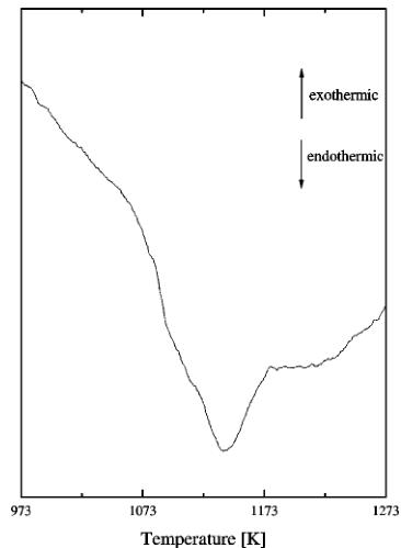
3.4. Transition to the Cubic Form
The phase transition at 1140.15 K was thought to be of the first order. However, this hypothesis should be dismissed as the calorimetric trace of the transition presented in Fig. 8 does not have the characteristic sharp onset of the peak and steep fall of the DTA signal caused by absorption of the transition heat. It is also unusually broad while the first-order transformations, at constant pressure, have very well-defined transition temperature. The transition causes a large change in the heat capacity. The heat corresponding to the area of the peak is around 40.9 J/g, which is probably the reason that it was thought to be the first order. Also the previous incorrect choice of the perovskite unit cell gave an artificial decrease in the unit cell volume upon the transition. With the new model the difference in volume of the cell before and after the transformation is only \( V(1173.15\ \text{K}) - V(1073.15\ \text{K}) = 0.098\ \text{\AA}^{3} \) and can be accounted for by the thermal expansion of the material.

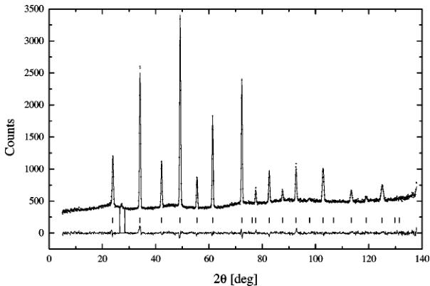
FIG. 6. An example of refined cubic pattern at 1223.15 K.
behavior of the oxide within the transition range is peculiar and the diffraction pattern collected at 1148.15 K contains the cubic and the orthorhombic phases. The material had been kept for 15 min at this temperature before the measurement, so what we are looking at is most likely the equilibrium state. The diffraction pattern is presented in Fig. 9. The two-phase character of the pattern is not obvious at first, but careful examination of peak intensities and comparison with the single-phase patterns leads to this conclusion. All cubic reflections overlap heavily with the orthorhombic peaks. The pattern was refined as a two-phase spectrum and

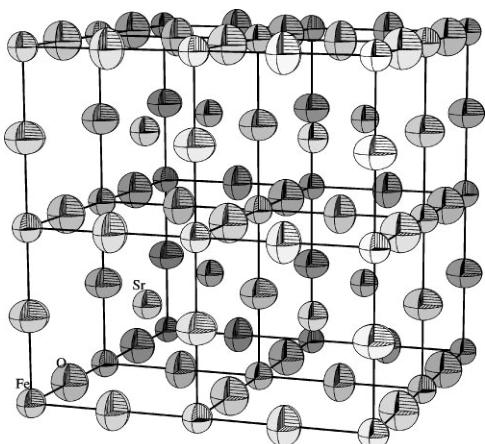
FIG. 7. The cubic unit cell at 1123.15 K. The ellipsoids represent thermal motion of atoms and correspond to 50% probability surfaces.
yielded fractions of the cubic \( f_{c}=0.373 \) and the orthorhombic \( f_{o}=0.627 \) phases, respectively. Due to the overlap, the results for this pattern are less reliable than those for the single-phase ones. However, the extreme values of cell volumes of both phases do not cause large changes in the volume of the sample. The weighted average cell volume (average volume occupied by four molecules) is only \( f_{o}V_{o}+f_{c}V_{c}=505.02\mathring{A}^{3} \) , which is not far from volumes of the single-phase samples before and after the transformation. The two-phase pattern indicates that the transition from the

FIG. 8. The DTA trace of the second-phase transition in \( Sr_{2}Fe_{2}O_{5} \)

FIG. 9. The refined two-phase pattern at 1148.15 K.
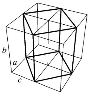
orthorhombic form to cubic is continuous. Its mechanism is actually quite simple. The orthorhombic structure itself contains distorted cubic cells. The pseudo-cubic cells can be clearly seen if we divide the crystal into identical blocks larger than the unit cell as shown in Fig. 10. The block has the same height as the orthorhombic lattice constant b. The base of the block is made out by the diagonals of bases of four adjacent orthorhombic cells. The pseudo-cell has twice the volume of the orthorhombic unit cell and splits at \( y = \frac{1}{2} \) into two cubic cells upon the transition. The dimensions and angles between the edges of the block are close to parameters of the cube. The ratio of the base edge length \( \sqrt{a^{2} + c^{2}} \) to the half of the height b/2 is close to one. Also the acute angle of the rhombus base exceeds \( 88^{\circ} \) (it is the acute angle between the diagonals of the orthorhombic

FIG. 10. A schematic division of the orthorhombic lattice into blocks containing two distorted cubic cells. Letters denote the orthorhombic unit cell edges.
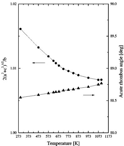
base). The changes of these parameters with temperature are presented in Fig. 11. The edge ratio slowly decreases with temperature, reaching the value of 1.0082 at 1103.15 K; at the same time the angle approaches the value of 88.76°. The content of the cell derived from the refinement results at 1073.15 K is presented in Fig. 12. As discussed previously, iron and oxygen ions are connected and strontium is shown as unconnected spheres. The block consists of layers of iron ions in octahedral Fe(1) and tetrahedral Fe(2) sites divided

FIG. 11. The cell edge ratios and angles of the distorted cubic cells as a function of temperature.

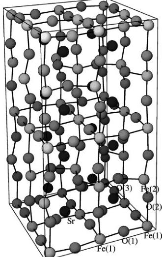
FIG. 12. The fragment of the orthorhombic crystal structure at 1073.15 K obtained by the division shown in Fig. 10. Oxygen and iron ions are connected; strontium is represented by unconnected spheres.
by layers of oxygen O(2). Oxygen O(1) lies slightly off the plane containing the octahedral iron. Oxygen O(3) occupies the planes at \( y = \frac{1}{4} \) and \( y = \frac{3}{4} \) . The block can be subdivided into 16 distorted perovskite cells. All of them contain strontium in the middle. The transition from the orthorhombic to the cubic phase is just a matter of small changes in the atom positions in the unit cell.
ACKNOWLEDGMENTS
The authors thank Dr. Andrew J. Studer, of the Australian Nuclear Science and Technology Organisation, for his help with collection of the neutron diffraction patterns. We thank Dr. Wojciech Schmidt of the Institute of Molecular Physics, Polish Academy of Sciences, for his valuable discussion of the magnetic structure results. We also acknowledge the financial support of the project by the Australian Institute of Nuclear Science and Engineering.
REFERENCES
-
B. C. H. Steele, Curr. Opin. Solid State Mater. Sci. 1, 684–691 (1996).
-
P. K. Gallagher, J. B. MacChesney, and D. N. E. Buchanan, J. Chem. Phys. 41, 2429–2434 (1964).
-
T. Takeda, Y. Yamaguchi, H. Watanabe, S. Tomiyoshi, and H. Yamamoto, J. Phys. Soc. Jpn. 26, 1320 (1969).
-
Z. Friedman, H. Shaked, and S. Shtrikman, Phys. Lett. 25A, 9–10 (1967).
-
T. Takeda, Y. Yamaguchi, S. Tomiyoshi, M. Fukase, M. Sugimoto, and H. Watanabe, J. Phys. Soc. Jpn. 24, 446–452 (1968).
-
C. Greaves, A. J. Jacobson, B. C. Tofield, and B. E. F. Fender, Acta Crystallogr. B31, 641–646 (1975).
-
M. Harder and Hk. Müller-Buschbaum, Z. Anorg. Allg. Chem. 464, 169–175 (1980).
-
H. Watanabe, J. Phys. Soc. Jpn. 12, 515–522 (1957).
-
J.-C. Grenier, N. Ea, M. Pouchard, and P. Hagenmuller, J. Solid State Chem. 58, 243–252 (1985).
-
S. Shin, M. Yonemura, and H. Ikawa, Mater. Res. Bull. 13, 1017–1021 (1978).
-
Y. Takeda, K. Kanno, T. Takada, and O. Yamamoto, J. Solid State Chem. 63, 237–249 (1986).
-
J. Mizusaki, M. Okayasu, S. Yamaguchi, and K. Fueki, J. Solid State Chem. 99, 166–172 (1992).
-
R. Knott, Neutron News 9, 23–32 (1998).
-
A. C. Larson and R. B. Von Drele, “GSAS General Structure Analysis System” Los Alamos National Laboratory Report, LAUR 86-748, 1994.
-
H. M. Rietveld, J. Appl. Crystallogr. 2, 65–71 (1969).
-
M. J. Cooper and J. P. Sayer, J. Appl. Crystallogr. 8, 615–618 (1975).
-
M. W. Thomas, J. Appl. Crystallogr. 10, 12–13 (1977).
-
G. Caglioti, A. Paoletti, and F. P. Ricci, Nucl. Instrum. 3, 223–228 (1958).
-
W. Marshall and S. W. Lovesey, “Theory of Thermal Neutron Scattering. The Use of Neutrons for the Investigation of Condensed Matter,” p. 471. Clarendon, Oxford, 1971.
-
JCPDS-ICDD PDF File No. 33-677.
-
A. I. Vogel, “A Text-Book of Macro and Semimicro Qualitative Inorganic Analysis,” 4th ed., p. 262. Longmans, New York, 1954.
-
M. Schmidt and S. J. Campbell, submitted.
-
M. A. Alario-Franco, J. C. Joubert, and J. P. Lévy, Mater. Res. Bull. 17, 733–740 (1982).
-
M. A. Alario-Franco, J. M. Gonzalez-Calbet, and M. Vallet-Regi, J. Solid State Chem. 49, 219–231 (1983).
-
M. Vallet-Regi, J. M. Gonzalez-Calbet, J. Verde, and M. A. Alario-Franco, J. Solid State Chem. 57, 197–206 (1985).
-
J. M. González-Calbet, M. Vallet-Regi, and M. A. Alario-Franco, J. Solid State Chem. 60, 320–331 (1985).
-
N. Nakayama, M. Takano, S. Inamura, N. Nakaishi, and K. Kosuge, J. Solid State Chem. 71, 403–417 (1987).
-
M. Takano, T. Okita, N. Nakayama, Y. Bando, Y. Takeda, O. Yamamoto, and J. B. Goodenough, J. Solid State Chem. 73, 140–150 (1988).
 p10_0.jpg
 p11_0.jpg
 p11_1.jpg
 p11_2.jpg
 p12_0.jpg
 p12_1.jpg
 p12_2.jpg
 p13_0.jpg
 p3_0.jpg
 p3_1.jpg
 p4_0.jpg
 p7_0.jpg
 p7_1.jpg