Marinite Li_{2}M(SO_{4}){2} (M = Co, Fe, Mn) and Li{1}Fe(SO_{4})_{2}: Model Compounds for Super-Super-Exchange Magnetic Interactions

Marine Reynaud, \( ^{\dagger} \) Gwenaëlle Rousse, \( ^{*,\ddagger} \) Jean-Noël Chotard, \( ^{\dagger} \) Juan Rodríguez-Carvajal, \( ^{\S} \) and Jean-Marie Tarascon \( ^{\dagger} \)

\( ^{\dagger} \) Laboratoire de Réactivité et Chimie des Solides (LRCS), Université de Picardie Jules Verne, CNRS UMR 7314, 33 rue Saint Leu, 80039 Amiens cedex, France

\( ^{\ddagger} \) Institut de Minéralogie et de Physique des Milieux Condensés (IMPMC), Université Pierre et Marie Curie, UPMC Univ Paris 06, CNRS UMR 7590, 4 Place Jussieu, 75252 Paris cedex 05, France

\( ^{8} \) Institut Laue-Langevin (ILL), BP 156, 6 rue Jules Horowitz, 38042 Grenoble cedex 9, France

Supporting Information

ABSTRACT: New materials initially designed for battery electrodes are often of interest for magnetic study, because their chemical compositions include 3d transition metals. We report here on the magnetic properties of marinite phases \( \mathrm{Li}_{2}\mathrm{M}(\mathrm{SO}_{4})_{2} \) (M = Fe, Co, Mn) and \( \mathrm{Li}_{1}\mathrm{Fe}(\mathrm{SO}_{4})_{2} \) , which all order antiferromagnetically at low temperature. From neutron powder diffraction, we propose a model for their ground-state magnetic structures. The magnetism of marinite \( \mathrm{Li}_{2}\mathrm{M}(\mathrm{SO}_{4})_{2}^{\cdot} \) compounds unambiguously results from super-super-exchange interactions; therefore, these materials can be considered as a model case for which the Goodenough–Kanamori–Anderson rules can be tested.

■ INTRODUCTION

Since the discovery of \( LiFePO_{4} \) as a promising positive electrode material for Li-ion batteries, \( ^{1} \) there has been a growing interest in polyanionic compounds among the battery research community, and numerous new materials have been proposed. \( ^{2-4} \) In this context, our group has been reporting over the years on a wide family of fluorosulfates, with general formula \( AMSO_{4}F \) (A = Li, Na; M = Fe, Co, Ni, Mn, Zn, Mg). \( ^{5-12} \) Among them, the favorite and triplet forms of \( LiFeSO_{4}F \) have drawn particular attention, because they display the highest potentials ever obtained for the \( Fe^{III+}/Fe^{II+} \) redox couple in inorganic compounds (3.6 and 3.9 V versus \( Li^{+}/Li^{0} \) , respectively). \( ^{5,8,10} \) Following this work, we investigated the bimetallic sulfates and we isolated two new compounds— \( Li_{2}M(SO_{4})_{2} \) (M = Fe, Co)—among which the iron phase also demonstrates a high potential of 3.83 V vs \( Li^{+}/Li^{0} \) for the \( Fe^{III+}/Fe^{II+} \) redox couple. \( ^{13} \) We recently prepared the manganese equivalent \( Li_{2}Mn(SO_{4})_{2} \) which is presented herein along with the accurate structural determination of the delithiated \( Li_{1}Fe(SO_{4})_{2} \) phase.

Aside from being attractive electrode materials for Li-ion batteries, these new \( \mathrm{Li_{2}M(SO_{4})_{2}} \) (x = 1, 2; M = Fe, Co, Mn) phases can constitute model compounds for magnetic studies as the particular arrangement of \( MO_{6} \) octahedra and \( SO_{4} \) tetrahedra of their structure should solely enable super-super-exchange interactions. Among polyanionic compounds, few iron-based materials (e.g., \( FePO_{4} \) \( ^{14} \) , \( Fe_{2}(SO_{4})_{3} \) \( ^{15,16} \) , \( Fe_{2}(MoO_{4})_{3} \) \( ^{17} \) , \( Li_{3}Fe_{2}(PO_{4})_{3} \) \( ^{18,19} \) , \( LiFeP_{2}O_{7} \) \( ^{20} \) , \( AFe(SO_{4})_{2} \) (A = K, Cs,

Rb) \( ^{21,22} \) present such singular structures in which interactions between magnetic atoms are only possible via M–O–O–M pathways. They generally lead to antiferromagnetic long-range ordering, \( ^{14-20} \) but can also result in more-complex magnetic structures (e.g., helical) due to topologically frustrated interactions. \( ^{21,22} \) Other works compare the magnetism of different 3d metals within isostructural sulfate-based compounds, in which both M–O–M super-exchange interactions and M–O–O–M super-super-exchange interactions are likely to occur. One can cite, in particular, the works on the antiferromagnetic anhydrous metal sulfates \( MSO_{4} \) (M = Fe, Ni, Co), \( ^{23} \) on the antiferromagnetic fluorosulfates \( AMSO_{4}F \) (A = Li, Na; M = Fe Co), \( ^{7,12,24} \) on the ferrimagnetic hydroxysulfates \( M_{3}(OH)_{2}(SO_{4})_{2}(H_{2}O)_{2} \) (M = Co, Mn, Ni), \( ^{25-27} \) and on the jarosite \( AM_{3}(SO_{4})_{2}(OH)_{6} \) (A = Na, K, Ag, Rb, H, \( NH_{4} \) etc.; M = Fe, Cr, V) whose Kagomé lattice leads to strong frustration and exotic magnetic structures. \( ^{28-30} \)

We present here a detailed report on the temperature-dependent magnetic susceptibility of the four marinite compounds \( \mathrm{Li_{2}Co^{II}(SO_{4})_{2}} \) , \( \mathrm{Li_{2}Mn^{II}(SO_{4})_{2}} \) , \( \mathrm{Li_{2}}Fe^{II}(SO_{4})_{2} \) , and \( \mathrm{Li_{1}}Fe^{III}(SO_{4})_{2} \) , and we further use low-temperature neutron powder diffraction to determine their magnetic structures. Finally, we perform an analysis of the super-super-exchange

---

interactions and discuss the relative strengths required to obtain the observed magnetic structures as the ground state.

EXPERIMENTAL SECTION

Sample Preparation. The \( \mathrm{Li_{2}M(SO_{4})_{2}} \) samples (M = Co, Fe, Mn) were prepared following the previously reported procedure \( ^{13} \) which consists of three steps: (i) stoichiometric amounts of \( Li_{2}SO_{4} \) and \( MSO_{4} \) are thoroughly mixed using a Spex Miller 8000M, (ii) the resulting powder is pressed into a pellet, (iii) the latter is annealed at \( 325\ ^{\circ}C \) for 12–48 h, either under air (M = Co, Mn) or in a quartz tube sealed under vacuum (M = Fe). In contrast to the Fe phase, neither the Co compound nor the Mn compound are electrochemically active, with respect to Li metal. Thus, only the delithiated phase \( \mathrm{Li_{2}Fe(SO_{4})_{2}} \) was obtained through chemical oxidation of \( \mathrm{Li_{2}Fe(SO_{4})_{2}} \) , using an excess of \( NO_{2}BF_{4} \) (>2 equiv) as an oxidizing agent in acetonitrile.

Structural Characterization. Purity of the samples was checked by laboratory powder X-ray diffraction (XRD), with a Bruker D8 diffractometer equipped with an X-ray tube providing Cu Kα radiation and a LynxEye detector.

Neutron powder diffraction (NPD) was performed on the D2B and D20 diffractometers at the Institut Laue Langevin (ILL, Grenoble, France). The D2B diffractometer has a very high resolution and, therefore, was used to precisely refine the nuclear structure of \( Li_{1}Fe(SO_{4})_{2} \) at room temperature, using a wavelength of \( \lambda = 1.594 \) Å. The high-intensity D20 diffractometer has a good resolution at low angles and was used to determine the magnetic structures of the title compounds. NPD patterns on D20 were recorded either under high-flux conditions (takeoff angle = \( 42^{\circ} \) ), using a wavelength of \( \lambda = 2.418 \) Å, or in the high-resolution mode (takeoff angle = \( 90^{\circ} \) ) with two different wavelengths ( \( \lambda = 1.543 \) and \( 2.416 \) Å).

Synchrotron powder X-ray diffraction data ( \( \lambda = 0.4139 \) Å) were obtained through the mail-in service of the 11-BM beamline at the Advanced Photon Source (Argonne National Laboratory, Argonne, IL, USA).

Nuclear and magnetic structures were refined using the Rietveld method \( ^{31} \) as implemented in the FullProf program. \( ^{32,33} \) For the magnetic structure determination, Bertaut symmetry analyses \( ^{34} \) were carried out using the program BasIReps within the same suite of software. The structures were drawn and examined with the help of the FullProf Studio program, as well as the VESTA visualization program. \( ^{35} \)

Magnetic measurements. Susceptibility measurements were carried out using either a SQUID SS or a SQUID XL magnetometer (Quantum Design), in zero-field-cooled (ZFC) and field-cooled (FC) modes, under applied magnetic fields of 10 kOe and 100 Oe. Magnetization curves \( (M = f(H)) \) were recorded at 2 K. Powder samples of roughly 20–30 mg were placed into gel caps for the measurement.

■ RESULTS

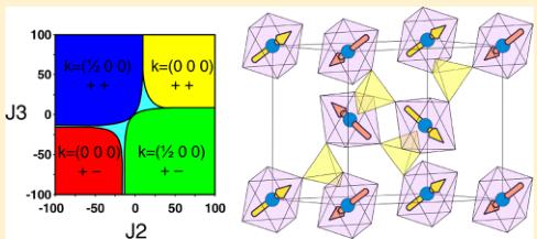
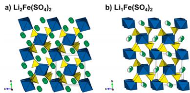
Crystal Structures. We reported on the synthesis, electrochemical properties, and structures of the new \( \mathrm{Li_{2}Co(SO_{4})_{2}} \) and \( \mathrm{Li_{2}Fe(SO_{4})_{2}} \) compounds in a previous communication. \( ^{13} \) Unlike the lithium nickel sulfate \( \mathrm{Li_{2}Ni(SO_{4})_{2}} \) , which has an orthorhombic structure \( (Pbca) \) , \( ^{36} \) the cobalt and iron analogues crystallize in a monoclinic unit cell (space group \( P2_{1}/c \) ). Their structure is built upon \( MO_{6} \) octahedra, which are connected to each other through their six vertices by \( SO_{4} \) tetrahedra (Figure 1a). Each sulfate tetrahedron is linked to three different \( MO_{6} \) octahedra; its fourth corner points to a large tunnel along the a-axis, in which the Li atoms sit.

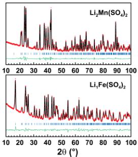
Later, we were able to synthesize a manganese equivalent \( \mathrm{Li_{2}Mn(SO_{4})_{2}} \) using the same procedure as the one previously described for the cobalt analogue. The high similarity of their two XRD patterns suggested that this new lithium manganese sulfate crystallizes in the same structure as the iron and cobalt compounds. This was confirmed with a Rietveld refinement of

Figure 1. Comparison of the structures of (a) \( \mathrm{Li_{2}Fe(SO_{4})_{2}} \) and (b) \( \mathrm{Li_{1}Fe(SO_{4})_{2}} \) . Projections along the a-axis. \( FeO_{6} \) octahedra and \( SO_{4} \) tetrahedra are displayed in blue and yellow, respectively. The Li atoms are shown as green balls. In the delithiated phase, the lithium is on a half-occupied site as represented by the half-colored balls.

the XRD data, whose results are given in the Supporting Information (Figure SI-1 and Table SI-1).

We previously reported the lattice parameters of \( \mathrm{Li_{1}Fe(SO_{4})_{2}} \) , prepared by chemical delithiation from \( \mathrm{Li_{2}Fe(SO_{4})_{2}} \) , but X-ray laboratory data were not ideal to precisely determine the structure, and, in particular, the position of the Li atoms within the unit cell. \( ^{13} \) To accurately determine its crystal structure, we performed NPD on the high-resolution powder diffractometer D2B at ILL (Grenoble, France) using a wavelength of \( \lambda = 1.594 \) Å. Starting from a refinement of the NPD pattern of \( \mathrm{Li_{1}Fe(SO_{4})_{2}} \) and using the \( FeO_{6} \) octahedra and \( SO_{4}^{-} \) tetrahedra framework pertaining to \( \mathrm{Li_{2}Fe(SO_{4})_{2}} \) structure, we were able to precisely localize the position of the Li atoms in the center of the channels described above, using Fourier differential maps calculations, which were performed with the GFourier program of the FullProf Suite \( ^{32,33} \) (Figure SI-2a). Refinement of the structure with one Li atom placed in the special position \( \left(^{1}/_{2}0^{1}/_{2}\right) \) (2d Wyckoff site) resulted in an important anisotropic displacement (equivalent isotropic temperature factor \( B \approx 8 \mathring{A}^{2} \) ), with the main direction of the ellipsoid elongated along \( \langle 5 1 2 \rangle \) (see Figure SI-2b in the Supporting Information). This suggested that the Li ions are more likely distributed on a general position 4e located in the vicinity of the 2d position, with half occupancy. This led to a much lower temperature factor \( B \approx 1.1 \mathring{A}^{2} \) ). The resulting position of Li is shown in Figures SI-2c and SI-2d in the Supporting Information. The two half-occupied positions for Li around the \( \left(^{1}/_{2}0^{1}/_{2}\right. \) site are then separated by a distance of 0.7 Å, which is consistent with the anisotropic displacement calculated with the first model. Finally, a joint refinement of the structure was performed against both D2B NPD data and 11-BM Synchrotron XRD data. The results of this refinement are presented in the Supporting Information (Figure SI-3 and Table SI-2). A bond valence sum analysis, using \( b_{0} \) parameters from Brown, \( ^{37} \) indicates that the Fe–O bond lengths are in excellent agreement with iron in the III+ oxidation state, also confirmed by Mössbauer data (see the Supporting Information, Figure SI-4). As a result, the structure of \( \mathrm{Li_{1}Fe(SO_{4})_{2}} \) ; presents the same framework of \( FeO_{6} \) octahedra and \( SO_{4}^{+} \) tetrahedra as the lithiated phase (Figure 1b), but the octahedra and tetrahedra in \( \mathrm{Li_{1}Fe(SO_{4})_{2}} \) are slightly tilted compared to \( \mathrm{Li_{2}Fe(SO_{4})_{2}} \) . After the removal of one Li ion, the remaining Li ion of \( \mathrm{Li_{1}Fe(SO_{4})_{2}} \) . shifts toward the middle of the tunnel in a split position with half occupancy. As a consequence, the Li ions are coordinated by five O atoms, which is more preferable than the highly elongated octahedral coordination that lithium would adopt in the \( \left(^{1}/_{2}0^{1}/_{2}\atop2d\ \mathrm{Wyckoff\ position}\right) \) . Moreover, this five-coordination is geometrically similar to the coordination of the lithium in the pristine \( \mathrm{Li_{2}Fe(SO_{4})_{2}} \) compound.

---

In short, the four studied compounds \( (\mathrm{Li}_{2}\mathrm{Co}(\mathrm{SO}_{4})_{2}, \mathrm{Li}_{2}\mathrm{Mn}(\mathrm{SO}_{4})_{2}, \mathrm{Li}_{2}\mathrm{Fe}(\mathrm{SO}_{4})_{2}) \) , and \( \mathrm{Li}_{1}\mathrm{Fe}(\mathrm{SO}_{4})_{2}) \) present the same framework of \( MO_{6} \) octahedra and \( SO_{4} \) tetrahedra, in which the metal atoms are all isolated from each other and are only interconnected through the sulfate tetrahedra. Such a specific connectivity suggests that the magnetic properties are only due to super-super-exchange interactions, hence our interest to study the magnetic properties of these materials as described next.

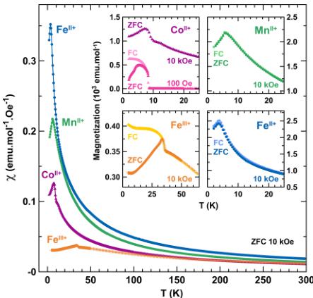
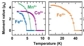
Magnetic Properties. The macroscopic magnetic properties of the title compounds were determined with a SQUID magnetometer in both ZFC and FC conditions under 10 kOe. Curves of the temperature dependence of the ZFC magnetic susceptibility are shown in Figure 2. All compounds show cusps

Figure 2. Temperature dependence of the magnetic susceptibility ( \( \chi \) ) of the title compounds, measured under zero-field-cooled (ZFC) conditions with a field of 10 kOe between 300 and 2 K. Purple triangles, green squares, orange crosses, and blue circles are assigned to \( \mathrm{Li}_{2}\mathrm{Co}^{\mathrm{II}}(\mathrm{SO}_{4})_{2} \) , \( \mathrm{Li}_{2}\mathrm{Mn}^{\mathrm{II}}(\mathrm{SO}_{4})_{2} \) , \( \mathrm{Li}_{1}\mathrm{Fe}^{\mathrm{II}}(\mathrm{SO}_{4})_{2} \) and \( \mathrm{Li}_{2}\mathrm{Fe}^{\mathrm{II}}(\mathrm{SO}_{4})_{2} \) respectively. Insets show enlargement of the ZFC (dark colors) and field-cooled (FC) (light colors) magnetization curves at low temperatures. For \( \mathrm{Li}_{2}\mathrm{Co}^{\mathrm{II}}(\mathrm{BO}_{4})_{2} \) only the 10-kOe ZFC curve is shown (purple triangles) and compared to the ZFC (dark pink) and FC (light pink) curves measured with a field of 100 Oe.

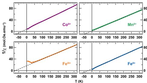
of a long-range antiferromagnetic ordering, which occurs at a Néel temperature \( (T_{\mathrm{N}}) \) of \( \sim7 \) K for \( \mathrm{Li}_{2}\mathrm{Co}^{\mathrm{II}}(\mathrm{PO}_{4})_{2} \) , \( \sim6 \) K for \( \mathrm{Li}_{2}\mathrm{Mn}^{\mathrm{II}}(\mathrm{PO}_{4})_{2} \) , \( \sim4 \) K for \( \mathrm{Li}_{2}\mathrm{Fe}^{\mathrm{II}}(\mathrm{PO}_{4})_{2} \) , and \( \sim35 \) K for \( \mathrm{Li}_{1}\mathrm{Fe}^{\mathrm{III}}(\mathrm{PO}_{4})_{2} \) . The high-temperature region (200–300 K) of the inverse susceptibility was fitted to the Curie–Weiss equation \( \chi = C/(T - \theta_{\mathrm{CW}}) \) (see Figure 3). We deduced the Curie–Weiss temperatures to be approximately \( -30 \) K, \( -8 \) K, \( -23 \) K, and \( -71 \) K, and the effective moments were determined to be \( 5.4 \mu_{\mathrm{B}} \) , \( 5.9 \mu_{\mathrm{B}} \) , \( 5.7 \mu_{\mathrm{B}} \) , and \( 5.8 \mu_{\mathrm{B}} \) for \( \mathrm{Li}_{2}\mathrm{Co}^{\mathrm{II}}(\mathrm{O}_{4})_{2} \) , \( \mathrm{Li}_{2}\mathrm{Mn}_{\mathrm{II}}^{\mathrm{II}}(\mathrm{PO}_{4})_{2} \) , \( \mathrm{Li}_{2}\mathrm{Fe}^{\mathrm{II}}(\mathrm{BO}_{4})_{2} \) , and \( \mathrm{Li}_{1}\mathrm{Fe}^{\mathrm{III}}(\mathrm{BO}_{4})_{2} \) , respectively. These results are summarized in Table 1, together with the frustration parameter \( |\theta_{\mathrm{CW}}|/T_{\mathrm{N}} \) .

Usually, the value of the effective moment of a given cation can be calculated using the following formula: \( \mu_{\mathrm{eff}} = g_{1} \cdot [J(J + 1)]^{1/2} \) , where \( g_{1} \) is the Landé gyromagnetic factor and J is the total angular momentum (the sum of the spin angular momentum S and the orbital angular momentum L). However, the effective moment is often affected by the crystal field and thus differs from the expected value for the free ion. Two models are actually used

Figure 3. Evolution of the inverse of the magnetic susceptibility \( (1/\chi) \) of the title compounds as a function of the temperature. Purple, green, orange, and blue colors are assigned to \( \mathrm{Li}_{2}\mathrm{Co}^{\mathrm{II}}\left(\mathrm{SO}_{4}\right)_{2} \) , \( \mathrm{Li}_{2}\mathrm{Mn}^{\mathrm{III}}\left(\mathrm{SO}_{4}\right)_{2} \) , \( \mathrm{Li}_{1}\mathrm{Fe}^{\mathrm{III}}\left(\mathrm{SO}_{4}\right)_{2} \) , and \( \mathrm{Li}_{2}\mathrm{Fe}^{\mathrm{II}}\left(\mathrm{SO}_{4}\right)_{2} \) , respectively. Experimental curves are fitted with the ideal Curie–Weiss law in the temperature range of 200 K \( \leq T \leq 300 \) K (dashed lines).

to account for this phenomenon: (i) the orbital moment L may be fully decoupled from the spin contribution S (i.e., the spin–orbit coupling L·S is null), thus leading to an effective moment given by the equation \( \mu_{\mathrm{eff}} = [4S(S + 1) + L(L + 1)]^{1/2} \) ; (ii) the orbital contribution L may be completely quenched and the system would then present a spin-only effective moment, which is calculated from the formula \( \mu_{\mathrm{eff}} = 2 \cdot [S(S + 1)]^{1/2} \) (or \( \mu_{\mathrm{eff}} = [n(n + 2)]^{1/2} \) , with n being the number of unpaired electrons). Table 1 shows that the experimental effective moments deduced from the magnetic measurements of \( \mathrm{Li}_{2}\mathrm{Co}^{\mathrm{II}}(\mathrm{VO}_{4})_{2} \) and \( \mathrm{Li}_{2}\mathrm{Be}^{\mathrm{II}}(\mathrm{SO}_{4})_{2} \) are consistent with the expected effective moment of a single 3d metal cation in a high-spin octahedral environment with an unquenched orbital moment, which is fully decoupled from the spin contribution. However, one should note that the case of \( Co^{II} \) is always pretty tricky, as high-spin \( Co^{II} \) samples are known to exhibit significant spin–orbit coupling that manifests itself in the population of the Kramers \( S = \pm^{1/2} \) doublet ground state, and these samples can be regarded as carrying an effective spin of \( S = ^{1/2} \) with a large Landé factor. We cannot rule out such a possibility and further experiments such as EPR or magnetization measurements on single crystals could be of interest. In fact, as discussed below, the refined magnetic moment of \( Co^{II} \) ions (3.3 \( \mu_{B} \) ) is slightly higher than the spin-only value ( \( 3.0 \mu_{B} \) ). In the case of \( \mathrm{Li}_{2}\mathrm{Mn}^{\mathrm{II}}(\mathrm{VO}_{4})_{2} \) and \( \mathbf{Li}_{1}\mathbf{Fe}^{\mathrm{III}}(\mathrm{SO}_{4})_{2} \) , the orbital moment is null and the experimental values for the effective moment are in good agreement with a spin-only effective moment calculated for a \( d^{5} \) transition metal.

The inset of Figure 2 shows an enlargement of the magnetization curves at low temperatures for ZFC and FC measurements under 10 kOe, as well as the ZFC/FC curves for the \( Co^{II} \) -based sample under 100 Oe. \( \mathrm{Li}_{2}\mathrm{Mn}^{\mathrm{II}}(\mathrm{BO}_{4})_{2} \) and \( \mathrm{Li}_{2}\mathrm{Re}^{\mathrm{II}}(\mathrm{SO}_{4})_{2} \) present a typical antiferromagnetic behavior, with the ZFC and FC curves that are superimposed. Concerning \( \mathrm{Li}_{1}\mathrm{Fe}^{\mathrm{III}}(\mathrm{SO}_{4})_{2} \) , the ZFC and FC curves deviate at temperatures below \( T_{N} \) , which may result from either a ferromagnetic impurity or some ferromagnetic/ferrimagnetic contributions. Since neither the XRD nor the NPD patterns reveal the presence of a secondary phase, the latter hypothesis is more probable. A similar behavior is observed for \( \mathrm{Li}_{2}\mathrm{Co}^{\mathrm{II}}(\mathrm{S}\mathrm{O}_{4})_{2} \) , with, in addition, a nonlinearity of the moment versus the applied field, as the curves recorded under a field of 100 Oe lead to magnetization larger than expected from the value obtained at 10 kOe.

---

Table 1. Magnetic Parameters of the Title Compounds Deduced from Magnetic Measurements and Neutron Diffraction, and Compared to Some Expected Theoretical Values

	Li4CoII(SO4)2	Li2MnII(SO4)2	Li3FeII(SO4)2	Li1FeII(SO4)2
electronic configuration	d7:t2g5e2	d5:t2g5e2	d6:t2g4e2	d5:t2g5e2
	S = 3/2, L = 3	S = 5/2, L = 0	S = 2, L = 2	S = 5/2, L = 0
Experimental Values Deduced from Magnetic Measurements (H = 10 kOe)
Néel temperature, TN	7 K	6 K	4 K	35 K
Curie constant, C	3.7 emu K mol−1	4.3 emu K mol−1	4.1 emu K mol−1	4.3 emu K mol−1
Curie–Weiss temperature, θCW	−30 K	−8 K	−23 K	−71 K
frustration parameter, |θCW|/TN	4.29	1.33	5.75	2.03
effective moment, μeff	5.4 μB	5.9 μB	5.7 μB	5.8 μB
Experimental Values Deduced from Neutron Diffraction
Néel temperature, TN	8 K	6 K	5 K	39 K
magnetic moment at 1.85 K	3.3 μB	4.6 μB	3.2 μB	4.3 μB
Expected Theoretical Values
effective moment, μeff
μeff = g·[J(J + 1)]1/2	6.6 μB	5.9 μB	6.7 μB	5.9 μB
μeff = [4S(S + 1) + L(L + 1)]1/2	5.2 μB	5.9 μB	5.5 μB	5.9 μB
μeff = 2·[S(S + 1)]1/2	3.9 μB	5.9 μB	4.9 μB	5.9 μB
magnetic moment, m = g·S	3 μB	5 μB	4 μB	5 μB

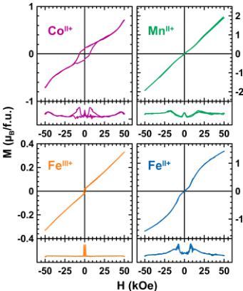
Figure 4. Magnetization curves of \( \mathrm{Li_{2}Co^{II}(SO_{4})_{2}} \) (purple), \( \mathrm{Li_{2}Mn^{II}(SO_{4})_{2}} \) (green), \( \mathrm{Li_{3}Fe^{III}(SO_{4})_{2}} \) (orange), and \( \mathrm{Li_{3}Fe^{II}(SO_{4})_{2}} \) (blue), as a function of the applied field measured at 2 K. Derivative curves are displayed in the lower part of each diagram.

To test this point, we recorded the magnetization curves at 2 K for the four samples (Figure 4). The magnetization curve of \( \mathrm{Li_{2}Co^{II}(SO_{4})_{2} \) clearly shows a hysteresis loop, which indicates a weak ferromagnetic behavior with a remnant magnetization \( (M_{\mathrm{t}}) \) of \( 0.12 \mu_{B} \) and a coercive field \( (H_{\mathrm{c}}) \) of 6.5 kOe. This can explain the discrepancy between the ZFC and FC curves previously mentioned. Close inspection of the data for \( \mathrm{Li_{2}Mn^{II}(SO_{4})_{2}} and \mathrm{Li_{3}Fe^{III}(SO_{4})_{2}} \) also reveals a tiny weak ferromagnetism, and the remnant magnetization is \( \sim0.02 \mu_{B} \) . The absence of any hysteresis loop on the magnetization curve of \( \mathrm{Li_{2}Fe^{II}(SO_{4})_{2}} \) confirms a pure antiferromagnetic ground state, which is consistent with the ZFC/FC curves that are neatly superimposed. Switching to higher fields, the evolution of the magnetization of \( \mathrm{Li_{3}Fe^{III}(SO_{4})_{2}} is linear with the applied field, while an interesting feature is observed for \( \mathrm{Li_{2}Fe^{II}(SO_{4})_{2}} and \mathrm{Li_{2}Co^{II}(SO_{4})_{2}} \) . The magnetization for the latter presents an inflection point of \( \sim45 \) kOe (seen in the derivative curve in Figure 4), which may suggest a metamagnetic behavior; therefore, this point must be confirmed by magnetization measurements at higher field for checking the feasibility to saturate the magnetization, and single-crystal experiments would be needed to confirm this. A similar inflection point can be seen for the \( Fe^{II} \) -based compound, but the field at which it occurs is much lower ( \( \sim10 \) kOe); therefore, this could result from a canted magnetic structure that becomes colinear under the effect of the magnetic field. To figure this out, we embarked into an NPD study to determine the magnetic structures of each counterpart.

Magnetic Structures. NPD measurements were performed on the four title compounds at the D20 diffractometer of the Institut Laue-Langevin (ILL). With a high resolution at low \( 2\theta \) angles, the D20 diffractometer is a choice instrument for magnetic structure determination. NPD patterns of the \( \mathrm{Li_{2}(SO_{4})_{2}} \) and \( \mathrm{Li_{2}Fe(SO_{4})_{2}} \) samples were acquired in a high flux configuration using a \( \lambda = 2.418 \AA \) wavelength, while the newly reported \( \mathrm{Li_{2}Mn(SO_{4})_{2}} \) and \( \mathrm{Li_{1}Fe(SO_{4})_{2}} \) phases were measured in high-resolution mode at two different wavelengths: \( \lambda = 1.543 \AA \) and \( \lambda = 2.416 \AA \) .

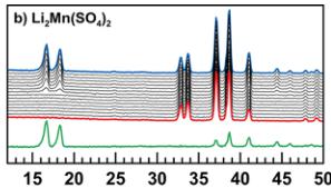
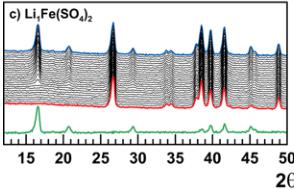
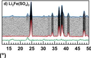
Crystallographic data obtained from the Rietveld refinement of the NPD patterns acquired above the Neel temperature of each compound are summarized in Tables 2–5, and the results of these refinements for \( \mathrm{Li_{2}Mn(SO_{4})_{2}} \) are presented in Figure 5. Upon cooling the powder samples (Figure 6), we observed the growth of new peaks, which indicates a long-range ordering of the magnetic moments. These extra peaks are better observed when plotting the difference patterns (green lines in Figure 6) of a diagram recorded above \( T_{N} \) (red patterns in Figure 6) and of another one recorded below \( T_{N} \) (blue patterns in Figure 6).

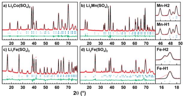
Next, NPD patterns were recorded at 1.85 K in order to determine the magnetic structure of each compound. We found that the magnetic reflections observed for \( \mathrm{Li_{2}Co(SO_{4})_{2}} \) , \( \mathrm{Li_{2}Mn(SO_{4})_{2}} \) , and \( \mathrm{Li_{1}Fe(SO_{4})_{2}} \) can be indexed in the same unit cell as their nuclear structure. The propagation vector is the gamma-point of the Brillouin zone: \( \mathbf{k} = (0, 0, 0) \) . A symmetry analysis was then performed using Bertaut's method, \( ^{34} \) as implemented in the program BasIReps in order to determine all possible spin configurations compatible with the crystal symmetry of the nuclear structure. The results of this analysis are

---

Table 2. Nuclear and Magnetic Structures of \( Li_{2}Co(SO_{4})_{2} \) . Results from a Bond Valence Sum Analysis \( ^{37} \) (BVS) are Reported

Nuclear Structure
D20 Diffractometer in High-Flux Mode, \( \lambda = 2.418 \) Å, T = 15 K
space group: \( P2_{1}/c \)			\( R_{\text{Bragg}} = 1.86\% \) , \( \chi^{2} = 76.7 \)
a = 4.9671(2) Å, b = 8.0908(3) Å, c = 8.7639(3) Å, \( \beta = 121.855(5)^{\circ} \) , V = 299.162(17) Å \( ^{3} \)
atom	Wyckoff position	occupancy	x	y	z
Co	2a	1.0	0	0	0
Li	4e	1.0	0.014 (3)	0.6352(12)	0.1015(18)
S	4e	1.0	0.3388(18)	0.3021(12)	0.3046(10)
O1	4e	1.0	0.1810(13)	0.4176(5)	0.1507(6)
O2	4e	1.0	0.2005(10)	0.1342(7)	0.2463(5)
O3	4e	1.0	0.2861(9)	0.3510(4)	0.4465(5)
O4	4e	1.0	0.6854(9)	0.3018(4)	0.3764(5)
Magnetic Structure
D20 Diffractometer in High-Flux Mode; \( \lambda = 2.418 \) Å, T = 1.85 K
k = (0, 0, 0), \( \Gamma_{3} \)
atom	\( M_{x} \) ( \( \mu_{B} \) )	\( M_{y} \) ( \( \mu_{B} \) )	\( M_{z} \) ( \( \mu_{B} \) )	\( M_{\text{tot}} \) ( \( \mu_{B} \) )
Co (0 0 0)	0.12	3.33(3)	0	3.33(3)
Co (0 \( \frac{1}{2} \) \( \frac{1}{2} \) )	0.12	-3.33(3)	0	3.33(3)	0

Table 3. Nuclear and Magnetic Structures of \( Li_{2}Mn(SO_{4})_{2} \) . Results from a Bond Valence Sum Analysis \( ^{[37]} \) (BVS) are Reported

Nuclear Structure
D20 Diffractometer in High-Resolution Mode, \( \lambda = 1.543 \) Å, T = 15 K
space group: \( P2_{1}/c \(			\) R_{\text{Bragg}} = 3.38\%, \chi^{2} = 16.4 \(
a = 4.9811 (1) Å, b = 8.3140 (2) Å, c = 8.8382 (2) Å, \) \beta = 121.250 (5) \( ^{\circ}, V = 312.910 (9) \) Å \( ^{3} \)
atom	Wyckoff position	occupancy	x	y	z
Mn	2a	1.0	0	0	0.66 (8)
Li	4e	1.0	0.0175 (16)	0.6299 (8)	0.1044 (9)
S	4e	1.0	0.3286 (10)	0.3026 (6)	0.2975 (6)
O1	4e	1.0	0,1756 (6)	0.4145 (3)	0.1497 (3)
O2	4e	1.0	0,1928 (5)	0.1391 (3)	0.2449 (3)
O3	4e	1.0	0,2886 (6)	0.3533 (3)	0.4448 (3)
O4	4e	1.0	0,6711 (6)	0.2980 (3)	0.3630 (3)
Magnetic Structure
D20 Diffractometer in High-Resolution Mode; \( \lambda = 2.416 \) Å, T = 1.85 K
k = (0, 0, 0), \( \Gamma_{1} \)
atom	\( M_{x} \) ( \( \nu_{B} \) )	\( M_{y} \) ( \( \nu_{B} \) )	\( M_{z} \) ( \( \nu_{B} \) )	\( M_{\text{tot}} \) ( \( \nu_{B} \) )
Mn (0 0 0)	3.97 (8)	0.02	-1.03 (12)	4.59 (18)
Mn (0 \( \frac{1}{2} \) \( \frac{1}{4} \) )	-3.97 (8)	0.02	1.03 (12)	4.59 (18)

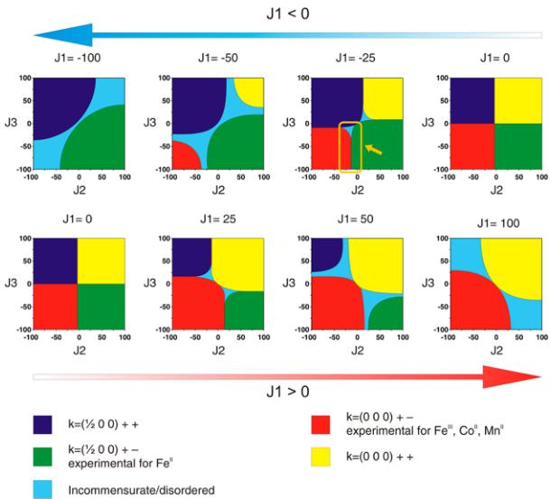
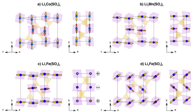
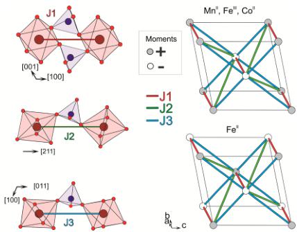
summarized in Table 6. Two irreducible representations were found to be associated with the 2a Wyckoff site (0 0 0) which is occupied by the 3d metals: \( \Gamma_{magetic} = 3\Gamma_{1} + 3\Gamma_{3} \) . These representations are built with three basis vectors which are collinear to the a, b, and c unit cell directions, respectively. In the \( \Gamma_{1} \) representation, the magnetic moments of the two metal atoms, which are nonrelated by lattice translations ( \( M_{1} \) in (0 0 0) and \( M_{2} \) in (0 \( \frac{1}{2} \) \( \frac{1}{3} \) ) are constrained to be \( (u, v, w) \) and \( (-u, v, -w) \) for \( M_{1} \) and for \( M_{2} \) , respectively. The corresponding Shubnikov group is \( P2_{1}/c \) . In the \( \Gamma_{3} \) representation, the directions of the magnetic moments of the \( M_{1} \) and \( M_{2} \) atoms become of the form \( (u, v, w) \) and \( (u, -v, w) \) , respectively. The corresponding Shubnikov group is \( P2_{1}^{\prime}/c^{\prime} \) . For the three phases \( Li_{2}Co(SO_{4})_{2} \) , \( Li_{2}Mn(SO_{4})_{2} \) , and \( Li_{1}Fe(SO_{4})_{2} \) , we tested all the possibilities given by these two irreducible representations against the NPD patterns recorded at 1.85 K, and we determined the magnetic structure for each compound. First, we found that the magnetic moments of \( Li_{2}Co(SO_{4})_{2} \) align antiferromagnetically along the b-axis, as allowed by the \( \Gamma_{3} \) representation. In agreement with the SQUID measurements, a weak ferromagnetic component can be added in the \( (ac) \) plane, since it is indeed allowed by symmetry; however, because of the weakness of these ferromagnetic components, they cannot be refined from NPD data. The results of this refinement are shown in Figure 7a and in the lower part of Table 2. The refined value of the magnetic moment of the cobalt is then \( 3.33(3) \) \( \mu_{B} \) . The magnetic structure of \( Li_{2}Co(SO_{4})_{2} \) is illustrated in Figure 8a. It shows the alternate orientations \( (+ -) \) of the moments along the [011] direction while the sequence of the moments is \( (+ +) \) along the [100] and [001] directions.

Unlike the cobalt phase, the best agreement with the magnetic reflections observed for \( \mathrm{Li_{2}Mn(SO_{4})_{2}} \) and \( \mathrm{Li_{1}Fe(SO_{4})_{2}} \) was obtained using the irreducible representation \( \Gamma_{1} \) . For the manganese analogue, a magnetic moment aligned along the a-

---

Table 4. Nuclear and Magnetic Structures of \( Li_{1}Fe(SO_{4})_{2} \) . Results from a Bond Valence Sum Analysis \( ^{37} \) (BVS) are Reported

} \endtable> Table 5. Nuclear and Magnetic Structures of \( Li_{2}Fe(SO_{4})_{2} \) . Results from a Bond Valence Sum Analysis\(^{37}\) (BVS) are Reported

Nuclear Structure
D20 Diffractometer in High-Resolution Mode, \( \lambda = 1.543 \) Å, \( T = 50 \) K
space group: \( P2_{1}/c \)				\( R_{\text{Bragg}} = 2.67\% \) , \( \chi^{2} = 13.5 \)
a = 4.7974(2) Å, b = 8.3815(2) Å, c = 7.8956(2) Å, \( \beta = 121.835(5)^{\circ} \) , V = 269.721(10) ų
atom	Wyckoff position	occupancy	x	y	z	B_{\text{iso}} (Ų)
Fe	2a	1.0	0	0	0	0.31(6)
Li	4e	0.5	0.581(5)	0.025(3)	0.524(4)	1.5(5)
S	4e	1.0	0.2974(16)	0.1797(7)	0.7592(8)	0.09(12)
O1	4e	1.0	0.0413(7)	0.1296(4)	0.7985(4)	0.25(7)
O2	4e	1.0	0.2602(8)	0.1067(4)	0.5871(5)	0.30(7)
O3	4e	1.0	0.2876(7)	0.3564(4)	0.7391(5)	0.36(7)
O4	4e	1.0	0.3781(7)	0.6428(4)	0.5594(5)	0.53(7)
Magnetic Structure
D20 Diffractometer in High-Resolution Mode
k = (0, 0, 0), \( \Gamma_{1} \)
atom	\( M_{x} \) ( \( \mu_{B} \) )	\( M_{y} \) ( \( \mu_{B} \) )	\( M_{z} \) ( \( \mu_{B} \) )	\( M_{tot} \) ( \( \mu_{B} \) )
Fe (0 0 0)	0	0.02	4.33(4)	4.33(4)
Fe (0 1/2 1/2)	0	0.02	-4.33(4)	4.33(4)

Nuclear Structure
D20 Diffractometer in High-Flux Mode, \( \lambda = 2.418 \) Å, \( T = 10 \) K
space group: \( P2_{1}/c \(				\( R_{\text{Bragg}} = 6.4\% \) , \( \chi^{2} = 87.4 \)
a = 4.9836(7) Å, b = 8.1910(13) Å, c = 8.8108(11) Å, \( \beta = 121.915(9)^{\circ} \) , V = 305.30(7) ų
atom	Wyckoff position	occupancy	x		y	z
Fe	2a	1.0	0		0	0
Li	4e	1.0	0.020(5)	0.645(3)	0.102(4)	1.11(4)
S	4e	1.0	0.334(5)	0.293(3)	0.315(3)	5.83(17)
O1	4e	1.0	0	0.183(3)	0.4139(10)	1.66(6)
O2	4e	1.0	0	0.194(2)	0.1379(12)	2.19(9)
O3	4e	1.0	0	0.2841(16)	0.3569(8)	0.4482(11)
O4	4e	1.0	0	0.6884(19)	0.3016(8)	0.3782(12)
Magnetic Structure
D20 Diffractometer in High-Flux Mode, \( \lambda = 2.41 \) Å, \( T = 1.85 \) K
k = (1/2, 0, 0), \( \Gamma_{1} \)
Atom	\( M_{x} \) ( \( \mu_{B} \) )	\( M_{y} \) ( \( \mu_{B} \) )		\( M_{z} \) ( \( \mu_{B} \) )		\( M_{\text{tot}} \) ( \( \mu_{B} \) )
Fe (0 0 0)	2.97(6)	1.25(10)		0		3.23(12)
Fe (0 1/2 1/2)	-2.97(6)	1.25(10)		0		3.23(12)

axis provides a rather good fit of the magnetic reflections (hypothesis Mn-H1 in Figure 7b). However, adding a small antiferromagnetic component along the c-axis improves the fit of the (101) and (T03) reflections \( (2\theta = 46^{\circ} \) and \( 48.5^{\circ} \) , respectively) as shown in the right panel of Figure 7b (box Mn-H2). The value of the total magnetic moment was then refined to \( 4.59(18)\mu_{B} \) . Regarding \( \mathrm{Li_{1}Fe(SO_{4})_{2}} \) , we determined its moments to be aligned along the c-axis, with a magnitude of \( 4.33(4)\mu_{B} \) . Note that a small peak at \( 2\theta = 18.5^{\circ} \) remains unindexed and may be attributed to an inhomogeneity of the sample or to a magnetic impurity. Finally, since SQUID measurement suggested a tiny weak-ferromagnetic behavior for both \( \mathrm{Li_{2}Mn(SO_{4})_{2}} \) and \( \mathrm{Li_{1}Fe(SO_{4})_{2}} \) , a small component of 0.02 \( \mu_{B} \) along the b-axis can be added to their magnetic moments, without any significant change on the refinement of the NPD data. The results of the refinements relative to the \( \mathrm{Li_{2}Mn(SO_{4})_{2}} \) ( \( \mathrm{Li_{1}Fe(SO_{4})_{2}} \) compounds are given at the bottom of Tables 3 and 4, and are illustrated in Figures 7b and 7c and Figures 8b and 8c, respectively. Since the propagation vector of \( \mathrm{Li_{2}Mn(SO_{4})_{2}} \) is the same as the one of \( \mathrm{Li_{2}Co(SO_{4})_{2}} \) (k = (0, 0, 0)), the spin sequence remains identical in the three compounds: (+) along the [011] and (+) along the [100] and [001]; the only difference lies in the orientation of the moments, as discussed previously. The same procedure was employed for the determination of the magnetic structure of \( \mathrm{Li_{2}Fe(SO_{4})_{2}} \) . However, although it crystallizes in the same crystal structure as the previous compounds, its magnetic reflections could not be indexed in the nuclear unit cell. Therefore, in this case, the propagation vector k was not \( (0, 0, 0) \) as it was for the other compounds, but it was found to be \( (^{1}/_{2}, 0, 0) \) , which results in a magnetic unit cell \( 2a \times b \times c \) , where a, b, and c are the unit-cell parameters of the nuclear structure. A symmetry analysis was then performed for \( k = (^{1}/_{2}, 0, 0) \) , and led to the two irreducible representations \( \Gamma_{1} \) and ---  Figure 5. Rietveld refinements of the neutron powder diffraction (NPD) patterns of \( Li_{2}Mn(SO_{4})_{2} \) and \( Li_{1}Fe(SO_{4})_{2} \) measured at 15 and 50 K, respectively, with a wavelength of 1.543 Å (D20 diffractometer). The red crosses and the black line represent the experimental and the calculated patterns, respectively. The green line is the difference curve of these two patterns. Bragg positions are shown as blue sticks. \( \Gamma_{3} \) , as described in Table 6. The representation \( \Gamma_{1} \) , with the basis vectors \( \{(1\ 0\ 0), (0\ 1\ 0), (0\ 0\ 1)\} \) for Fe1 and \( \{(T\ 0\ 0), (0\ 1\ 0), (0\ T)\} \) for Fe2, was found to give the best agreement with the observed magnetic peaks. This corresponds to the Shubnikov group \( P_{2d2} \) \( 1/c \) in the Opechowski–Guccione notation. \( ^{38} \) A first magnetic model was determined with all the magnetic moments being aligned along the a-axis. However, the refinement of this model did not result in a good fitting of all the magnetic peaks, as the intensity of the first satellite reflection at \( 2\theta = 16.4^{\circ} \) was not reproduced by this model (Figure 7d, right, box Fe-H1). Adding a magnetic component along the b-axis was finally found to fit well the neutron data (Figure 7d, right, box Fe-H2), leading to a non-collinear magnetic structure. The refined value of the magnetic moment of the iron is then \( 3.23(12)\mu_{\mathrm{B}} \) . The results of the refinement are summarized at the bottom of Table 5 and are displayed in Figures 7d and 8d. Thus, the propagation vector \( \mathbf{k} = (^{1}/_{2}, 0, 0) \) for \( \mathrm{Li}_{2}\mathrm{Fe}(\mathrm{SO}_{4})_{2} \) results in a different spin sequence from the ones observed for the other \( \mathrm{Li}_{x}\mathrm{M}(\mathrm{SO}_{4})_{2} \) compounds. In this case, the spins are parallel along the [010] and [001] directions and antiparallel along the [100] direction, while they are not collinear along the [011] direction. Therefore, we can retrospectively try to interpret the inflection point at 10 kOe observed in the magnetization curve for that compound (Figure 4): it is likely that this field is strong enough to align the magnetic moments, and the magnetic structure becomes collinear at higher field. Overall, the values of the magnetic moments obtained from the refinement of the magnetic structures of \( \mathrm{Li_{2}Mn(SO_{4})_{2}} \) ( \( Mn^{II+} \) : \( d^{5} \) , \( m_{exp} = 4.59 \mu_{B} \) , \( \mathrm{Li_{1}Fe(SO_{4})_{2}} \) ( \( Fe^{III+} \) : \( d^{5} \) , \( m_{exp} = -4.33 \mu_{B} \) ), and \( \mathrm{Li_{2}Fe(SO_{4})_{2}} \) ( \( Fe^{II+} \) : \( d^{6} \) , \( m_{exp} = 3.23 \mu_{B} \) ) are below the spin-only expected value ( \( g \cdot S = 5 \mu_{B} \) and \( 4 \mu_{B} \) for the \( d^{5} \) and \( d^{6} \) ions, respectively), as seen in Table 1. The magnetic moment reduction may be due to one (or more) of the following reasons: (1) the moments are not fully saturated as these compounds present relatively low Néel temperatures, (2) covalency by electron transfer toward the anions, and (3) zero-point fluctuations of the antiferromagnetic ground state. Conversely, the experimental magnetic moment ( \( m_{exp} = 3.33 \mu_{B} \) ) for \( \mathrm{Li_{2}Co(SO_{4})_{2}} \) ( \( Co^{II+} \) : \( d^{7} \) ) is slightly larger than the theoretical value of \( 3 \mu_{B} \) , which indicates a small contribution of the orbital moment, as often observed for cobalt. \( ^{12,24} \) Finally, neutron diffraction patterns were recorded for each sample at small intervals of temperature from 2 K until the magnetic peaks vanished. Sequential refinements against these data were performed using the FullProf suite \( ^{32,33} \) in order to follow the evolution of the magnitude of the magnetic moment with the temperature. The results of these refinements are presented in Figure 9. The Néel temperature deduced from these measurements are in good agreement with the SQUID data, as seen in Table 1. ## ■ DISCUSSION To understand why \( \mathrm{Li}_{2}\mathrm{Fe}(\mathrm{SO}_{4})_{z} \) ( \( Fe^{II+} \) : \( d^{6} \) ) presents a magnetic structure whose spin sequence is completely different from the three other maritime \( \mathrm{Li}_{x}\mathrm{M}(\mathrm{SO}_{4})_{2}\mathrm{compounds} \) ( \( M = Fe^{III+} \) , \( Mn^{II+} \) , \( Co^{II+} \) and x = 1, 2), we have performed an analysis of the topology of the super-super-exchange interactions which govern the nature of the long-range magnetic ordering.     Figure 6. Evolution of the NPD patterns of (a) \( \mathrm{Li_{2}Co(SO_{4})_{2}} \) , (b) \( \mathrm{Li_{2}Mn(SO_{4})_{2}} \) , (c) \( \mathrm{Li_{1}Fe(SO_{4})_{2}} \) , and (d) \( \mathrm{Li_{2}Fe(SO_{4})_{2}} \) while cooling the sample to 2 K (2.42 Å). Blue patterns are measured at 2 K while the red ones are measured at (a) 12 K, (b) 10 K, (c) 50 K, and (d) 7 K, respectively. Black patterns correspond to intermediate temperatures. The green lines represent the difference curves between the blue and the red patterns for each sample, i.e., the magnetic contribution. --- Table 6. Results of the Representation Analysis of the \( P2_{1}/c \) Space Group for the Two Propagation Vectors \( \mathbf{k}=(0,0,0) \) and \( \mathbf{k}=(\mathbf{1}/\mathbf{2},0,0)^{\alpha} \)

k = (0, 0, 0)				k = (1/2, 0, 0)
Γ1(++++)	(x y z)	(-x y + 1/2 -z + 1/2)	Γ1(++++)	(x y z)	(-x y + 2/2 -z + 1/2)
Ψ1	(1 0 0)	(Γ 0 0)	Ψ1	(1 0 0)	(Γ 0 00)
Ψ2	(0 1 0)	(0 1 0)	Ψ2	(0 1 0)	(0 1 00)
Ψ3	(0 0 1)	(0 0 Γ)	Ψ3	(0 0 1)	(0 0 Γ0)
Γ3(+-+-)	(x y z)	(-x y + 1/2 -z +1/2)	Γ3(+-+-)	(x y z)	(-x y +1/2 -z +1/2)
Ψ1	(1 00)	(1 0 0)	Ψ1	(1 00)	(1 0 0)0
Ψ2	(0 1 0)0	(0 Γ 0)	Ψ2	(0 1 0)	(00 1 0)
Ψ3	(0 0 1	(0 0 1)	Ψ3	(0 0 1)	(0 01)

\( ^{a} \) The basis vectors \( \Psi_{i} \) (i = 1, 2, 3) of the two M-atoms related by the operators \( (x y z) \) and \( (-x y^{+1}/2 - z^{+1}/2) \) are given for each irreducible representation \( \Gamma_{j} \) (j = 1, 3). The sequence of plus and minus signs corresponds to the characters of the symmetry operators \( I, 2_{1}, -I \) , and c.  Figure 7. Refinements of the nuclear and magnetic parts of the NPD patterns measured at 1.85 K for (a) \( \mathrm{Li_{2}Co(SO_{4})_{2}} \) (b) \( \mathrm{Li_{2}Mn(SO_{4})_{2}} \) (c) \( \mathrm{Li_{1}Fe(SO_{4})_{2}} \) and (d) \( \mathrm{Li_{3}Fe(SO_{4})_{2}} \) . For each phase, the red crosses and the black line represent the experimental and the calculated patterns, respectively. The green line is the difference curve of these two patterns. The first line of blue sticks corresponds to the Bragg positions of the nuclear part, while the second line of blue sticks shows the positions of the expected reflections of the magnetic part. The H1 and H2 boxes on the right-hand side of panels (b) and (d) highlight the difference of fitting of the patterns, depending on the model chosen, as described in the text.  Figure 8. Nuclear and magnetic structures of (a) \( \mathrm{Li_{2}Co(SO_{4})_{2} \) (b) \( \mathrm{Li_{2}Mn(SO_{4})} \) (c) \( \mathrm{Li_{1}Fe(SO_{4})} \) and (d) \( \mathrm{Li_{2}Fe(SO_{4})_{2}} \) . Magnetic moments are represented by vectors through the 3d metal atoms. Yellow vectors represent positive moments, while the orange ones represent negative moments. For the sake of clarity, Li atoms are omitted. Inspection of the NPD patterns, as a function of temperature, shows that, regardless of the transition metal, no additional magnetic reflections develop below the onset of long-range order, so that the magnetic structures we determined can be seen as the ground state. An analysis was performed by using the two programs SIMBO and ENERMAG \( ^{39} \) to determine the relative ---  Figure 9. Temperature dependence of the moment value deduced from the sequential refinement of the magnetic structures against D20 NPD data between 2 K and 50 K for the title compounds \( Li_{2}Co^{II}(SO_{4})_{2} \) (purple), \( Li_{2}Mn^{II}(SO_{4})_{2} \) (green), \( Li_{1}Fe^{III}(SO_{4})_{2} \) (orange), and \( Li_{2}Fe^{II}(SO_{4})_{2} \) (blue). strengths and signs of the different super-super-exchange interactions which are required to produce the observed magnetic structures. The programs are described in detail by Khayati et al. \( ^{40} \) Here, we followed a procedure that was successfully applied to other iron phosphates and sulfates. \( ^{7,12,19,20,41} \) Three interactions \( J_{n} \) (n = 1, 2, 3) have to be considered between the transition-metal atoms (Figure 10). \( J_{1} \) is the shortest  Figure 10. Geometrical characteristics of the three super-super-exchange paths \( J_{1} \) , \( J_{2} \) , and \( J_{3} \) (left). The topology (i.e., how these three paths connect transition-metal atoms in the cell) is shown on the right (for the sake of clarity, only transition-metal atoms are shown). one (less than 5 Å for the M–M direct distance), and links two transition metals (M) along [100] (a) via two \( SO_{4} \) tetrahedra, so that \( J_{1} \) has a double exchange path. \( J_{2} \) and \( J_{3} \) link two M atoms via a single \( SO_{4} \) tetrahedra, the former along [211] ( \( a + b/2 + c/2 \) ) and the latter along [011] ( \( (b + c)/2 \) ). \( J_{2} \) and \( J_{3} \) both show a more linear M–O–O–M configuration; therefore, M–M direct distances are in the range of 6.0–6.2 Å. The geometric characteristics (distances, bond angles, and torsion angles) of the exchange paths for each compound are reported in the Supporting Information (Table SI-3), and the resulting topology is shown on the right-hand side of Figure 10. It clearly appears that \( J_{1} \) , \( J_{2} \) , and \( I_{3} \) form triangular networks, which may lead to frustration, if they have the same sign and strength. Therefore, we embarked on a study of their relative values, to obtain the observed magnetic structures as the ground state. Our analysis only deals with the spin sequence of the magnetic moments carried by the transition-metal atoms; it does not consider their spatial orientation. This is a consequence of the fact that this analysis neglects the magnetocrystalline anisotropy, which may play a role in these compounds, mostly for the cases in which \( L \neq 0 \) . The first ordered state is obtained by a calculation as a function of k (on the surface or inside the Brillouin zone) and the exchange integrals. This magnetic first ordered state is given by the eigenvector corresponding to the highest eigenvalue of the Fourier transform of the exchange integral matrix: \[ \xi_{i j}(\mathbf{k})=\sum_{I}J_{i j}(\mathbf{R}_{i})\mathrm{e}^{-2\pi i\mathbf{k}\cdot\mathbf{R}_{i}} \] where \(i\) and \(j\) refer to the magnetic atoms in a primitive cell, and \(J_{ij}(\mathbf{R}_{i})\) is the isotropic exchange interaction between the spins of the atoms \(i\) and \(j\) in unit cells separated by the lattice vector \(\mathbf{R}_{i}\). Our convention is that negative \(J_{ij}\) means antiparallel coupling (pair interaction energy: \(E_{ij} = -J_{ij}S_{i}\cdot S_{j}\)). The phase diagram is easily obtained using the program ENERMAG; \( ^{39} \) since the \( \xi_{ij}(\mathbf{k}, J_{1}, J_{2}, J_{3}) \) matrix contains many terms, and thus the eigenvalues are cumbersome to obtain by hand. The values of the three \( J_{n} \) terms (n = 1, 2, 3) were allowed to vary between -100 and +100, to map all possibilities for the relative values of exchange integrals. The resulting phase diagram is shown in Figure 11. We plot here cuts in the \( J_{2}-J_{3} \) planes, for different \( J_{1} \) values. These diagrams of the first ordered state indicate, for a given set of \( (J_{1}, J_{2}, J_{3}) \) values, the magnetic structure (propagation vector and sign sequence) that presents the lowest energy and therefore can be considered as the ground state if there is no further magnetic phase transition below the Néel temperature ( \( T_{N} \) ). First of all, we can notice wide domains for which we get incommensurate or disordered magnetic phases, especially when \( J_{1} \) is negative and \( J_{2} \) and \( J_{3} \) are of same relative values and signs, and when \( J_{1} \) is positive and \( J_{2} \) and \( J_{3} \) are opposite sign but have the same absolute values (regions along the \( J_{2}-J_{3} \) diagonals, colored in light blue). This comes as no surprise, considering the possible geometric frustration present in this system, as seen in the right-hand side of Figure 10. Apart from these domains, the system adopts more likely two propagation vectors with two different spin sequences between the magnetic moments in (0 0 0) and in \( (0^{1/2}, 1/2) \) . Therefore, four ordered magnetic structures are seen as ground states, depending on the relative values of \( J_{1}, J_{2} \) and \( J_{3} \) : \( \mathbf{k} = (0, 0, 0) \) with \( (+\mathbf{+}) \) and \( (+\mathbf{-}) \) , and \( \mathbf{k} = (1/2, 0, 0) \) with \( (+\mathbf{+}) \) , and \( (+\mathbf{-}) \) . For example, the ferromagnetic structure, characterized by \( \mathbf{k} = (0, 0, 0) \) and \( (+\mathbf{+}) \) is observed in the region for which all \( J_{n} \) (n = 1, 2, 3), are positive (yellow domains). At first sight, the experimentally deduced magnetic structure for \( \mathrm{Li}_{2}\mathrm{Fe}(\mathrm{SO}_{4})_{2} \) ( \( \mathbf{k} = (^{1}/_{2}, 0, 0) \) and \( (+\mathbf{-}) \) ) is observed as the ground state when \( J_{1} < 0 \) , \( J_{2} > 0 \) , and \( J_{3} < 0 \) (green domain). At the opposite, the \( \mathrm{Li}_{x}\mathrm{M}(\mathrm{SO}_{4})_{2} \) (M = \( Fe^{III+} \) , \( Co^{II+} \) , \( Mn^{II+} \) ) magnetic structures ( \( \mathbf{k} = (0, 0, 0) \) and $ (+\mathbf{-}) \) ) are calculated with the lowest energy when \( J_{1} > 0 \) , \( J_{2} < 0 \) , and \( J_{3} < 0 \) (red domain). However, closer inspection indicates that both structures can be obtained for \( J_{1} < 0 \) , \( J_{2} < 0 \) , and \( J_{\mathbf{3}} < 0 \) , and only a small decrease in \( J_{2} \) intensity (still being negative) can explain the change from \( \mathbf{k} = (0, 0, 0) \) and ( \( +\mathbf{-} \) ) to \( \mathbf{k} = (^{1}/_{2}, 0, 0) + (+\mathbf{-}) \) . Therefore, the maritime system more than likely resides in the region marked by an arrow in Figure 11. As a consequence, these results are in agreement with empirical Goodenough–Kanamori–Anderson rules, \( ^{42,43} \) which would predict the same negative sign for all three of these super-super-exchange interactions, whatever the transition metal and its oxidation state: \( \mathrm{d}^{5} \) ( \( Mn^{II+} \) , \( Fe^{III+} \) ), \( \mathrm{d}^{6} \) ( \( Fe^{II+} \) ), and \( \mathrm{d}^{7} \) ( \( Co^{II+} \) ). More-detailed theoretical and numerical (DFT calculations) approaches are needed to understand the peculiar magnetic behavior of \( \mathrm{Li}_{2}\mathrm{Fe}(\mathrm{SO}_{4})_{12} \) in the maritime series. ---  Figure 11. Phase diagram showing the influence of the values of the super-super-exchange integrals \( J_{n} \) on the ground-state magnetic structures of marinite \( \mathrm{Li}_{2}\mathrm{M}(\mathrm{SO}_{4})_{2} \) . The diagram is shown as cuts in the \( J_{2}-J_{3} \) plans, for different values of \( J_{1} \) , all varying between -100 and +100. The marinite domains are highlighted by an orange arrow. Turning to \( T_{N} \) values, it does not come as a surprise that \( T_{N} \) drastically increases as we move from \( \mathrm{Li}_{2}\mathrm{Fe}(\mathrm{SO}_{4})_{2} \) to \( \mathrm{Li}_{1}\mathrm{Fe}(\mathrm{SO}_{4})_{2} \) , because of the fact that \( d^{5}-d^{3} \) interactions are stronger than \( d^{6}-d^{6} \) ones, because of a greater \( \sigma \) character and a shortening of the Fe-Fe distance. Similarly, an increase in \( T_{N} \) was previously reported for \( LiFePO_{4} \) and \( LiFeSO_{4}F \) upon lithium removal. \( ^{74,41} \) The \( T_{N} \) values for the \( \mathrm{Li}_{2}\mathrm{M}^{\mathrm{II}}(\mathrm{SO}_{4})_{2} \) (M = Co, Fe, Mn) phases are nearly the same (within \( \pm3~K \) ), despite the different electronic contributions of divalent \( Co^{II+} \) , \( Mn^{II+} \) , and \( Fe^{II+} \) cations, in agreement with the fact that magnetic interactions are dominated by super-super-exchange interactions. Otherwise, one would expect the \( T_{N} \) value to be higher for \( Mn^{II+} \) and decrease as spins are added to the \( t_{2g} \) orbitals, as observed for the \( LiMSO_{4}F \) series, where magnetism is governed by super-exchange interactions. \( ^{7} \) ## ■ CONCLUSION In this paper, we have reported on the structures of the manganese analogue \( \mathrm{Li}_{2}\mathrm{Mn}(\mathrm{SO}_{4})_{2} \) and the delithiated phase \( \mathrm{Li}_{1}\mathrm{Fe}(\mathrm{SO}_{4})_{3} \) which were determined from X-ray diffraction (XRD) and neutron powder diffraction (NPD), thus completing the marinite series of compounds \( \mathrm{Li}_{2}\mathrm{M}(\mathrm{SO}_{4})_{2}\ (\mathrm{M}=\mathrm{Fe},\mathrm{Co}) \) . A careful study of their magnetic properties revealed that the four phases are antiferromagnetic, with the \( Co^{II+} \) , \( Mn^{II+} \) , and Fe \( ^{III+} \) -based analogues presenting a weak ferromagnetism, and the \( \mathrm{Li}_{2}\mathrm{Co}^{II}(\mathrm{SO}_{4})_{2} \) showing indications of a possible meta-magnetic behavior. Moreover, the magnetic structures of these compounds have been subsequently investigated using low-temperature NPD. The particular arrangement of \( MO_{6} \) octahedra and \( SO_{4} \) tetrahedra of their nuclear structure correspond to a topology prone to triangular frustration and enables only super-super-exchange interactions. We have established that the ground-state magnetic structures of \( \mathrm{Li}_{2}\mathrm{Co}(\mathrm{SO}_{4})_{2} \) , \( \mathrm{Li}_{2}\mathrm{Mn}(\mathrm{SO}_{4})_{3} \) and \( \mathrm{Li}_{1}\mathrm{Fe}(\mathrm{SO}_{4})_{4} \) are simple sequences of alternate spins (+ -) along the [011] direction, inscribed in the nuclear unit cell with a \( \mathbf{k}=(0,0,0) \) propagation vector. All magnetic structures can be explained with three negative super-super-exchange paths \( J_{1} \) , \( J_{2} \) , and \( J_{3} \) , in agreement with Goodenough-Kanamori-Anderson rules. The magnetic structure of \( \mathrm{Li}_{2}\mathrm{Fe}(\mathrm{SO}_{4})_{4} \) was determined to be slightly more complex, because it is non-collinear and displays a \( \mathbf{k}=(\mathbf{1}/\mathbf{2},0,0) \) propagation vector. This can be seen as a result of a decrease of intensity of the transversal integral of exchange \( J_{2} \) , with respect to the other members of the marinite series. ## ■ ASSOCIATED CONTENT ## Supporting Information Tables of crystal data and results of Rietveld refinements of \( Li_{2}Mn(SO_{4})_{2} \) and \( Li_{1}Fe(SO_{4})_{2} \) Mössbauer spectra of \( Li_{1}Fe(SO_{4})_{2} \) and geometrical characteristics of the super-super-exchange paths (PDF), as well as X-ray crystallographic information files (CIF), have been deposited as Supporting Information. This material is available free of charge via the Internet at http://pubs.acs.org. ## AUTHOR INFORMATION Corresponding Author \( ^{*} \) E-mail: gwenaelle.rousse@upmc.fr. ## Notes The authors declare no competing financial interest. ## ■ ACKNOWLEDGMENTS The authors would like to thank Thomas Hansen for his precious help in collecting neutron powder diffraction data on the diffractometers D2B and D20 at the Institut Laue Langevin (ILL, Grenoble, France). Use of the Advanced Photon Source at Argonne National Laboratory was supported by the U.S. --- Department of Energy, Office of Science, Office of Basic Energy Sciences, under Contract No. DE-AC02-06CH11357. The authors acknowledge Moulay T. Sougrati (Institut Charles Gerhardt, Montpellier, France) for conducting Mössbauer experiments. G.R. thanks Y. Klein and G. Radtke for fruitful discussions and the staff of the Low Temperature Physics platform (UPMC, Paris, France). M.R. acknowledges the French "Ministère de l'Enseignement Supérieur et de la Recherche" for her Ph.D. Grant. ## REFERENCES (1) Padhi, A. K.; Nanjundaswamy, K. S.; Goodenough, J. B. J. Electrochem. Soc. 1997, 144, 1188–1194. (2) Gong, Z.; Yang, Y. Energy Environ. Sci. 2011, 4, 3223–3242. (3) Melot, B. C.; Tarascon, J.-M. Acc. Chem. Res. 2013, 46, 1226–1238. (4) Masquelier, C.; Croguennec, L. Chem. Rev. 2013, DOI: 10.1021/cr3001862. (5) Recham, N.; Chotard, J.-N.; Dupont, L.; Delacourt, C.; Walker, W.; Armand, M.; Tarascon, J.-M. Nat. Mater. 2010, 9, 68–74. (6) Barpanda, P.; Chotard, J.-N.; Recham, N.; Delacourt, C.; Ati, M.; Dupont, L.; Armand, M.; Tarascon, J.-M. Inorg. Chem. 2010, 49, 7401–7413. (7) Melot, B. C.; Rousse, G.; Chotard, J.-N.; Ati, M.; Rodríguez-Carvajal, J.; Kemei, M. C.; Tarascon, J.-M. Chem. Mater. 2011, 23, 2922–2930. (8) Barpanda, P.; Ati, M.; Melot, B. C.; Rousse, G.; Chotard, J.-N. Doublet, M.-L.; Sougrati, M. T.; Corr, S. A.; Jumas, J.-C.; Tarascon, J.-M. Nat. Mater. 2011, 10, 772–779. (9) Ati, M.; Melot, B. C.; Rousse, G.; Chotar, J.-N.; Barpanda, P.; Tarascon, J.-M. Angew. Chem., Int. Ed. 2011, 50, 10574–10577. (10) Ati, M.; Melot, B. C.; Chotard, J.-N.; Rousse, G.; Reynaud, M.; Tarascon, J.-M. Electrochem. Commun. 2011, 13, 1280–1283. (11) Reynaud, M.; Barpanda, P.; Rousse, G.; Chotard, J.-N.; Melot, B. C.; Recham, N.; Tarascon, J.-M. Solid State Sci. 2012, 14, 15–20. (12) Melot, B. C.; Rousse, G.; Chotard, J.- N.; Kemei, M. C.; Rodríguez-Carvajal, J.; Tarascon, J.- M. Phys. Rev. B 2012, 85, 094415. (13) Reynaud, M.; Ati, M.; Melot, B. C.; Sougrati, M. T.; Rousse, G.; Chotard, J.-N.; Tarascon, J.-M. Electrochem. Commun. 2012, 21, 77–80. (14) Battle, P. D.; Cheetham, A. K.; Gleitzer, C.; Harrison, W. T. A.; Long, G. J.; Longworth, G. J. Phys. C: Solid State Phys. 1982, 15, L919–L924. (15) Long, G. J.; Longworth, G.; Battle, P.; Cheetham, A. K.; Thundathil, R. V.; Beveridge, D. Inorg. Chem. 1979, 18, 624–632. (16) Culvahouse, J. W. J. Magn. Magn. Mater. 1980, 21, 133–136. (17) Battle, P. D.; Cheetham, A. K.; Long, G. J.; Longworth, G. Inorg. Chem. 1982, 21, 4223–4228. (18) Rousse, G.; Rodríguez-Carvajal, J.; Wurm, C.; Masquelier, C. Chem. Mater. 2001, 13, 4527–4536. (19) Rousse, G.; Rodríguez-Carvajal, J.; Wurm, C.;Masquelier, C. Appl. Phys. A: Mater. Sci. Process. 2002, 74, s704–s706. (20) Rousse, G.; Rodríguez-Carvajal, J.; Wurm, C.; Massquelier, C. Solid State Sci. 2002, 4, 973–978. (21) Serrano-González, H.; Bramwell, S. T.; Harris, K. D. M.; Kariuki, B. M.; Nixon, L.; Parkin, I. P.; Ritter, C. J. Appl. Phys. 1998, 83, 6314–6316. (22) Serrano-González, H.; Bramwell, S. T.; Harris, C. D. M.; Kariuki, B. M.; Nixon, L.; Parkin I. P.; Ritter, C. Phys. Rev. B 1999, 59, 14451–14460. (23) Frazer, B. C.; Brown, P. J. Phys. Rev. 1962, 125, 1283–1291. (24) Melot, B. C.; Chotard, J.-N.; Rousse, G. Ati, M.; Reynaud, M.; Tarascon, J.-M. Inorg. Chem. 2011, 50, 7662–7668. (25) Vilminot, S.; Richard-Plouet, M.; André, G.; Swierczynski, D.; Bourée-Vigneron, F.; Kurmoo, M. Inorg. Chem. 2003, 42, 6859–6867. (26) Ben Salah, M.; Vilminot, S.; André, G.; Richard-Plouet, M.; Bourée-Vigneron, F.; Mihiri, T.; Kurmoo, M. Chem.—Eur. J. 2004, 10, 2048–2057. (27) Ben Salah, M.; Vilminot, S.; André, G.; Bourée-Vigneron, F.; Richard-Plouet, M.; Mihiri, T.; Kurmoo, M. Chem. Mater. 2005, 17, 2612–2621. (28) Wills, A. S.; Harrison, A. J. Chem. Soc., Faraday Trans. 1996, 92, 2161. (29) Wills, A. S. Can. J. Phys. 2001, 79, 1501–1510. (30) Nocera, D. G.; Bartlett, B. M.; Grohol, D.; Papoutsakis, D.; Shores, M. P. Chem.—Eur. J. 2004, 10, 3850–3859. (31) Rietveld, H. M. J. Appl. Crystallogr. 1969, 2, 65–71. (32) Rodríguez-Carvajal, J. FullProf Suite. Available at http://www.ill.eu/sites/fullprof/index.html. (33) Rodríguez-Carvajal, J. Physica B 1993, 192, 55–69. (34) Bertaut, E. F. J. Phys. Colloques 1971, 32, C1–462–C1–470. (35) Momma, K.; Izumi, F. J. Appl. Crystallogr. 2011, 44, 1272–1276. (36) Isasi, J.; Jaulmes, S.; Elfakir, A.; Quarton, M. Z. Kristallogr.—New Cryst. Struct. 2001, 216, 331–332. (37) Brown, I. D.; Altermatt, D. Acta Crystallogr., Sect. B: Struct. Sci. 1985, 41, 244–247. (38) Opechowski, W.; Guccione, R. Magnetic Symmetry. In Magnetism; Rado, G. T.; Suhl, H., Eds.; Academic Press: New York, London, 1965; Vol. II-A, pp 105–165. (39) Rodríguez-Carvajal, J. SIMBO, ENERMAG and PHASE DIAGRAM programs. Available within the examples of the CrysFML repository at http://forge.ill.eu/projects/crysfml/repository. (40) El Khayati, N.; Cherkaoui El Mourslí, R.; Rodríguez-Carvajal, J.; André, G.; Blanchard, N.; Bourée, F.; Collin, G.; Roisnel, T. Eur. Phys. J., B 2001, 22, 429–442. (41) Rousse, G.; Rodríguez-Carvajal, J.; Patoux, S.; Masquelier, C. Chem. Mater. 2003, 15, 4082–4090. (42) Goodenough, J. B. Phys. Rev. 1955, 100, 564–573. (43) Goodenough, J. B. J. Phys. Chem. Solids 1958, 6, 287–297.