| Transition Temperature | 33.4 K |
|---|---|
| Experiment Temperature | 4 K |
| Propagation Vector | k1 (0, 0, 0) |
| Parent Space Group | Fdd2 (#43) |
| Magnetic Space Group | Fd'd'2 (#43.227) |
| Magnetic Point Group | m'm'2 (7.4.23) |
| Lattice Parameters | 20.67800 8.40500 6.44600 90.00 90.00 90.00 |
|---|---|
| DOI | 10.1103/physrevb.92.024423 |
| Reference | G. Gitgeatpong, Y. Zhao, M. Avdeev, R.O. Piltz, T.J. Sato and K. Matan, Physical Review B (2015) 92. |
| Label | Element | Mx | My | Mz | |M| |
|---|---|---|---|---|---|
| Cu1 | Cu | 0.93 | 0.0 | 0.0 | 0.93 |
Magnetic structure and Dzyaloshinskii-Moriya interaction in the \(S = \frac{1}{2}\) helical-honeycomb antiferromagnet \(\alpha\)-Cu\(_{2}\)V\(_{2}\)O\(_{7}\)
G. Gitgeatpong, \( ^{1,2} \) Y. Zhao, \( ^{3,4} \) M. Avdeev, \( ^{5} \) R. O. Piltz, \( ^{5} \) T. J. Sato, \( ^{6} \) and K. Matan \( ^{1,2,*} \)
\( ^{1} \) Department of Physics, Faculty of Science, Mahidol University, Bangkok 10400, Thailand
\( ^{2} \) ThEP, Commission of Higher Education, Bangkok 10400, Thailand
\( ^{3} \) Department of Materials Science and Engineering, University of Maryland, College Park, Maryland 20742, USA
\( ^{4} \) NIST Center for Neutron Research, National Institute of Standards and Technology, Gaithersburg, Maryland 20899, USA
\( ^{5} \) Australian Nuclear Science and Technology Organisation, ANSTO, Locked Bag 2001, Kirrawee DC, NSW, Australia
\( ^{6} \) IMRAM, Tohoku University, Sendai, Miyagi 980-8577, Japan
(Received 9 February 2015; revised manuscript received 22 June 2015; published 23 July 2015)
Magnetic properties of the \( S = \frac{1}{2} \) antiferromagnet \( \alpha \) -Cu \( _{2} \) V \( _{2} \) O \( _{7} \) have been studied using magnetization, quantum Monte Carlo (QMC) simulations, and neutron diffraction. Magnetic susceptibility shows a broad peak at \( \sim \) 50 K followed by an abrupt increase indicative of a phase transition to a magnetically ordered state at \( T_{N} = 33.4(1) \) K. Above \( T_{N} \) , a fit to the Curie-Weiss law gives a Curie-Weiss temperature of \( \Theta = -73(1) \) K suggesting the dominant antiferromagnetic coupling. The result of the QMC calculations on the helical-honeycomb spin network with two antiferromagnetic exchange interactions \( J_{1} \) and \( J_{2} \) provides a better fit to the susceptibility than the previously proposed spin-chain model. Two sets of the coupling parameters \( J_{1}: J_{2} = 1:0.45 \) with \( J_{1} = 5.79(1) \) meV and \( 0.65:1 \) with \( J_{2} = 6.31(1) \) meV yield equally good fits down to \( \sim T_{N} \) . Below \( T_{N} \) , weak ferromagnetism due to spin canting is observed. The canting is caused by the Dzyaloshinskii-Moriya interaction with an estimated bc-plane component \( |D_{p}| \simeq 0.14J_{1} \) . Neutron diffraction reveals that the \( S = \frac{1}{2} \) Cu \( ^{2+} \) spins antiferromagnetically align in the \( Fd'd'2 \) magnetic space group. The ordered moment of \( 0.93(9)\mu_{B} \) is predominantly along the crystallographic a axis.
DOI: 10.1103/PhysRevB.92.024423
PACS number(s): 75.30.Cr, 75.25.−j, 75.10.Pq, 75.50.Ee
I. INTRODUCTION
Low-dimensional quantum magnetism has attracted much interest from both theoretical and experimental condensed matter physicists for many decades [1,2]. It is known that in a one-dimensional (1D) antiferromagnetic system, long-range order is absent even at zero temperature [3], leading to various fascinating magnetic ground states and phenomena at low temperatures such as the spin-Peierls state in \( CuGeO_{3} \) [4,5] and \( TiOCl \) [6,7], the singlet ground state in the alternating spin-chain system \( (\mathrm{VO})_{2}\mathrm{P}_{2}\mathrm{O}_{7} \) [8], the fractional spinon excitations in \( CuSO_{4} \) [5] \( D_{2}O \) [9], and the Bose-Einstein condensation (BEC) of magnons in the double spin-chain system \( TlCuCl_{3} \) [10], in which weakly interacting dimers are formed at low temperatures and BEC is realized as the field-induced three-dimensional (3D) magnetic ordering. However, some approximate 1D antiferromagnets exhibit long-range order with a remnant of quantum fluctuations in a form of quantum renormalization of spin waves [11,12]. Hence, in order to apprehend diverse physics of these low-dimensional quantum magnets, it is crucial to identify a spin network and relevant underlying interactions that consequently cause magnetic ordering and govern spin dynamics.
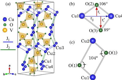
Among various compounds, copper-based oxides with \( Cu^{2+} \) ions \( (3d^{9}) \) , titanium-based oxides with \( Ti^{3+} \) ions \( (3d^{1}) \) , and vanadium-based oxides with \( V^{4+} \) ions \( (3d^{1}) \) are generally considered as a good realization of the low-dimensional spin- \( \frac{1}{2} \) system. Copper divanadate \( Cu_{2}V_{2}O_{7} \) is a promising realization of the low-dimensional spin- \( \frac{1}{2} \) system. There are two polymorphs of \( Cu_{2}V_{2}O_{7} \) that are generally found in a stable phase, namely the \( \alpha \) phase and the \( \beta \) phase with a structural phase transition at around \( 605^{\circ}C \) [14]. Other forms such as the \( \gamma \) and \( \beta' \) phases were also reported as complex and unstable high-temperature phases [14–16]. The \( \alpha \) phase of \( Cu_{2}V_{2}O_{7} \) crystallizes in the orthorhombic system of space group \( Fdd2 \) with \( a = 20.645(2) \) Å, \( b = 8.383(7) \) Å, and \( c = 6.442(1) \) Å [17,18]. Structurally, \( Cu^{2+} \) ions that are surrounded by five oxygen ions appear to form a chain of edge sharing \( CuO_{5} \) polyhedra while the nonmagnetic \( V^{5+} \) ions, each of which is surrounded by four oxygen ions to form \( V_{2}O_{7} \) double corner-sharing tetrahedra, are intercalated between the chains as shown in Fig. 1(a). Within the bc plane, the \( S = \frac{1}{2} \) spins of \( Cu^{2+} \) ions form a zigzag chain and interact with their nearest neighbors via two inequivalent Cu–O–Cu pathways. The distance between the two copper ions Cu1 and Cu4 connected by the blue bonds in Fig. 1(a) is approximately 3.1 Å. Intrachain interactions between these two copper ions are formed by the bridging of \( Cu1(Cu2) \) with \( Cu4(Cu3) \) along \( [011]([011]) \) via \( O(2) \) and \( O(3) \) . The deviation of the Cu–O(2)–Cu angle from \( 90^{\circ} \) [Fig. 1(b)] leads to a preferable and strong antiferromagnetic interaction along the chain [19]. In the previous study this system has been proposed as a realization of a zigzag spin-chain model [20]. However, the possibly strong next-nearest-neighbor interactions between the \( Cu^{2+} \) spins, which link the zigzag chains along the crystallographic a axis as shown by the green bonds in Fig. 1(a), suggest a highly anisotropic and nontrivial spin network with three coordinate spins for each site that resembles a disconnected honeycomb (helical-honeycomb) lattice when viewed along the b axis (Fig. 9). The next-nearest-neighbor bond of length 4.0 Å, which is slightly longer than the nearest-neighbor bond, is formed by the bridging of \( Cu1(Cu3) \) with \( Cu2(Cu4) \) via two equivalent \( O(1) \) ions [Fig. 1(c)]

FIG. 1. (Color online) (a) Crystal structure of \( \alpha \) -Cu \( _{2} \) V \( _{2} \) O \( _{7} \) . The chains of edge sharing CuO \( _{5} \) polyhedra are along [011] and [01 \( \bar{1} \) ] with two corner-sharing V \( _{2} \) O \( _{7} \) tetrahedra intercalated between the chains. Blue (J \( _{1} \) ) and green (J \( _{2} \) ) bonds represent the antiferromagnetic couplings between the nearest-neighbor, intrachain spins and next-nearest-neighbor, interchain spins, respectively. (b) The DM interactions, the directions of which can be determined from the cross product of \( r_{\perp} \times r_{ij} \) and \( r_{\perp}^{\prime} \times r_{ij} \) for two inequivalent Cu1–O(2)–Cu4 and Cu1–O(3)–Cu4 bonds, respectively, yield a nonzero value. (c) On the other hand, the equivalent Cu1–O(1)–Cu2 pathways connecting the interchain spins give rise to a net vanishing DM interaction. The structures are visualized using VESTA [13].
with the \( \mathrm{Cu-O(1)-Cu} \) angle of \( 104^{\circ} \) , possibly leading to an antiferromagnetic interaction that could be comparable to the intrachain interaction. This sizable interchain interaction that enables the forming of the helical-honeycomb lattice is not surprising. Using first-principle calculations on its cousin phase \( \beta-Cu_{2}V_{2}O_{7} \) , Tsirlin et al. [21] also suggested that the \( \beta \) phase could be better described by a honeycomb lattice than by a spin-chain model. The coordination number of three is the lowest for any two-dimensional (2D) lattices and only a 1D chain has a lower coordination number. Therefore, the helical-honeycomb model could share many properties unique to the low-dimensional magnets even though the lattice extends in three dimensions.
Magnetic susceptibility and heat capacity on a powder sample reveal that the antiferromagnet \( \alpha-Cu_{2}V_{2}O_{7} \) magnetically orders at a Néel temperature \( T_{N} \) of 34 K [20,22]. The magnetic ground state of \( \alpha-Cu_{2}V_{2}O_{7} \) was previously proposed to be a canted antiferromagnetic spin chain [20,22,23]. The canting of spins is due to Dzyaloshinskii-Moriya (DM) interactions, which give rise to the presence of weak ferromagnetism below \( T_{N} \) . However, the magnetic structure and spin dynamics of \( \alpha-Cu_{2}V_{2}O_{7} \) , have not been studied. Among the various probing techniques, neutron scattering is the most powerful at revealing the microscopic properties of such magnetic materials; however, a good quality large single crystal is required. Here we report the first detailed study of magnetic properties on single-crystal \( \alpha-Cu_{2}V_{2}O_{7} \) using magnetization, quantum Monte Carlo (QMC) simulations, and neutron diffraction measurements.
The paper is organized as follows. In Sec. II we briefly discuss single-crystal growth and experimental techniques used to characterize and study magnetic properties of the compound. The results in Sec. III are divided into three parts, where x-ray diffraction (Sec. III A), magnetization and QMC simulations (Sec. III B), and neutron diffraction (Sec. III C) will be discussed. Finally, we end with the summary in Sec. IV.
II. EXPERIMENTAL DETAILS
Prior to the single-crystal growth, powder \( Cu_{2}V_{2}O_{7} \) was prepared from high purity CuO and \( V_{2}O_{5} \) . The chemicals were dehydrated and weighed with stoichiometric ratio and then ground thoroughly with ethanol. The mixture was then calcined at \( 500^{\circ}C \) for 24 h. The obtained powder was inserted into a quartz tube. The bottom end of the tube was shaped into a taper for seed selection while the top end was tightly closed with silica wool. The sample was melted in air at \( 850^{\circ}C \) for 10 hours to ensure homogeneity and then lowered through a constant temperature gradient of about \( 40^{\circ}C/cm \) inside a vertical Bridgman furnace at a speed of 1 cm/day. The sample was finally cooled from \( 700^{\circ}C \) to room temperature at a rate of \( 5^{\circ}C/min \) . Single crystals were extracted from the quartz tube by mechanical separation. A pure-phase powder sample of \( \alpha-Cu_{2}V_{2}O_{7} \) was also synthesized by the standard solid state reaction and used in powder neutron diffraction measurements.
Small pieces of the crushed crystals were collected and ground for powder x-ray diffraction measurements using \( CuK\alpha \) radiation. The results were fit using the Rietveld method in FullProf [24]. To confirm the crystal structure, single-crystal x-ray diffraction data were collected at room temperature using a Bruker X8 APEX CCD diffractometer with \( MoK\alpha \) radiation. The refinements were done using the software ShelXle [25]. The magnetization M of the single-crystal sample was measured to the lowest temperature of 2 K using a superconducting quantum interference device (MPMS-XL, Quantum Design).
QMC simulations with the LOOP algorithm \( [26] \) were performed using the simulation package ALPS \( [27] \) . The magnetic susceptibility was calculated on a cluster of 100 spins for the spin-chain model and up to 432 spins (27 unit cells) for the helical-honeycomb model with a periodic boundary condition in the temperature range of \( 0.01 \leqslant t \leqslant 5 \) ( \( t = k_{B} T / J \) ) using 100 000 sweeps for thermalization and 500 000 Monte Carlo steps after thermalization.
To check crystallinity quality and investigate the magnetic transition, single-crystal neutron diffraction was performed at the BT7 Double Focusing Thermal Triple Axis Spectrometer [28] at NIST Center for Neutron Research, USA, on a single crystal with a mosaic of \( 0.8^{\circ} \) . Elastic neutron scattering were performed at 2.5 and 50 K using fixed incident energies of 14.7 and 30.5 meV. The position-sensitive detector (PSD) was employed in a two-axis mode with open– \( 80^{\prime\prime} \) –sample– \( 80^{\prime\prime} \) (radial)–PSD horizontal collimations to map out the broad reciprocal space in the \( (hk0) \) scattering plane [Fig. 6(a)]. A detailed investigation of the nuclear and magnetic Bragg reflections were performed using a triple-axis mode with a single detector and the horizontal collimations of open– \( 80^{\prime\prime} \) –sample– \( 80^{\prime\prime}-120^{\prime\prime} \) . For all diffraction measurements, one pyrolytic graphite (PG) filter and two PG filters were placed along the incident and scattered beams, respectively, to reduce higher-order neutron contamination. Neutron diffraction on the powder sample

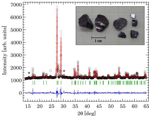
FIG. 2. (Color online) Powder x-ray diffraction was measured on crushed single crystals, black for the observed data, red for the calculated pattern, blue for the difference, and green for the Bragg positions. The symbols \( \star \) and \( \diamond \) indicate \( Cu_{0.64}V_{2}O_{5} \) and \( \beta-Cu_{2}V_{2}O_{7} \) impurities, respectively. The inset shows a photograph of the \( \alpha-Cu_{2}V_{2}O_{7} \) single crystals.
were performed at the high-resolution neutron diffractometer Echidna, ANSTO, Australia using neutrons with wavelength 2.44 Å (13.7 meV). The data were collected at 3 and 40 K to extract the magnetic scattering. Additional single-crystal neutron diffraction measurements were carried out at 4 and 50 K using the Laue diffractometer Koala, ANSTO, Australia. The Laue data images were processed using the LaueG software [29].
III. RESULTS AND DISCUSSION
A. X-ray diffraction
The obtained single crystals are shown in the inset of Fig. 2. The largest crystal was about \( 1 \times 1 \times 0.5 \, cm^{3} \) with a mass of 1.4 g. The naturally cleaved facet is the \( (1,0,0) \) plane. Small crystals were collected for the x-ray diffraction measurements, while large crystals were allocated for the neutron scattering experiments. The result of the powder x-ray diffraction (Fig. 2) shows that the major phase of the crystals is \( \alpha-Cu_{2}V_{2}O_{7} \) ( \( \sim 95\% \) ) with a small amount of impurities that can be identified as \( \beta-Cu_{2}V_{2}O_{7} \) and \( Cu_{0.64}V_{2}O_{5} \) [30]. We note that no trace of these impurities is detected in the powder sample (Fig. 7). The lattice constants obtained from the refinement are \( a = 20.678(6) \, \AA \) , \( b = 8.405(2) \, \AA \) , and \( c = 6.446(2) \, \AA \) , which are in good agreement with those reported in Ref. [18]. The impurities are still present after several crystal growth attempts with different cooling conditions, which are an important factor to control the ratio of \( \alpha \) and \( \beta \) phases [14,31]. We found that the fraction of \( \beta \) phase increases with an increasing cooling rate. Hence it is crucial to slowly cool the sample through the phase transition temperature at \( 605 \, ^{\circ}C \) to avoid a mixture of the two polymorphs. It should be noted that these impurities comprise only a small percentage, are most likely in a powder form, and hence will not mislead the interpretation of the neutron scattering data (Figs. 6 and 8). Room-temperature
TABLE I. Refined values of fractional coordinates of \(\alpha-\mathrm{Cu}_{2}\mathrm{V}_{2}\mathrm{O}_{7}\) from single-crystal x-ray diffraction measured at room temperature and from single-crystal neutron diffraction measured at 50 K.
| Atom | x/a | y/b | z/c | U |
| X-ray diffraction | ||||
| Cu | 0.16572(5) | 0.3646(1) | 0.7545(1) | 0.0143(3) |
| V | 0.19898(5) | 0.4055(1) | 0.2370(2) | 0.0067(3) |
| O(1) | 0.2455(3) | 0.5631(9) | 0.274(1) | 0.022(1) |
| O(2) | 0.1445(3) | 0.4375(6) | 0.0308(8) | 0.0100(9) |
| O(3) | 0.1617(3) | 0.3475(7) | 0.4575(9) | 0.014(1) |
| O(4) | \( \frac{1}{4} \) | \( \frac{1}{4} \) | 0.156(2) | 0.030(2) |
| \( R_{1}=0.039, wR_{2}=0.095, GOF=1.063 \) | ||||
| Neutron diffraction | ||||
| Cu | 0.16551(2) | 0.36460(5) | 0.7520(1) | 0.0036(1) |
| V | 0.1990(3) | 0.4046(8) | 0.237(2) | 0.0006(9) |
| O(1) | 0.24605(3) | 0.56165(8) | 0.2723(2) | 0.0072(2) |
| O(2) | 0.14428(3) | 0.43776(7) | 0.0286(2) | 0.0040(2) |
| O(3) | 0.16200(3) | 0.34608(9) | 0.4551(2) | 0.0052(2) |
| O(4) | \( \frac{1}{4} \quad \frac{1}{4} \) | \( \frac{1}{4} \quad 0.1507(3) \) | 0.0087(3) | |
| \( R_{1}=0.081, wR_{2}=0.073, GOF=1.215 \) | ||||
single-crystal x-ray diffraction was performed on the crystal a few hundreds of micrometers in size. The data were refined against space group \( Fdd2 \) with the previously reported lattice parameters [17] yielding the agreement factor \( R_{1}=0.039 \) for 1031 reflections with \( F_{\mathrm{obs}}<4\sigma(F_{\mathrm{obs}}) \) . The result is shown in Table I. The refinement result from single-crystal neutron diffraction measured at 50 K, which will be discussed later, is also shown in the table for comparison.
B. Magnetic susceptibility
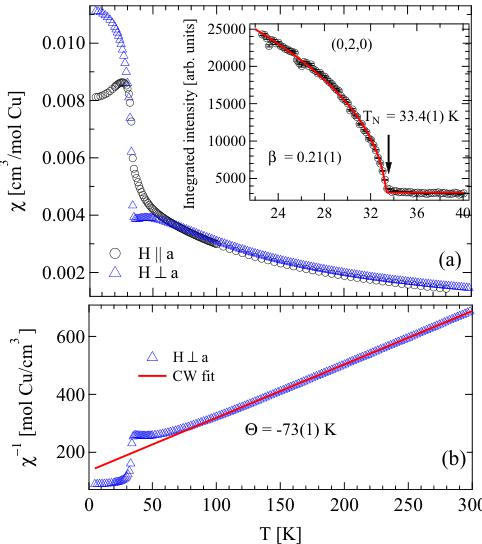
To investigate the magnetic transition on single-crystal \( \alpha-Cu_{2}V_{2}O_{7} \) , we measured the magnetic susceptibility ( \( \chi = M/H \) ) as a function of temperature when the applied magnetic field of 1 T was parallel and perpendicular to the a axis in the zero-field-cooled mode. In Fig. 3(a) the susceptibility exhibits clear anisotropy at low temperatures and shows a sharp transition at \( \simeq33 \) K in agreement with \( T_{N} = 33.4(1) \) K obtained from the order parameter measured by neutron diffraction on a single crystal at BT7 (the inset). The Néel temperature is consistent with that obtained from the susceptibility measured on our powder sample (not shown), as well as with those from the previous powder-sample studies [20,22].
Above 100 K, a linear fit of \( \chi^{-1} \) as a function of T to the Curie-Weiss law ( \( \chi = \frac{T}{C - \Theta} \) ) as shown in Fig. 3(b) gives a Curie-Weiss constant \( C = 0.545(2) \) cm \( ^{3} \) K/mol Cu and a Curie-Weiss temperature \( \Theta = -73(1) \) K. The negative Curie-Weiss temperature suggests that the dominant exchange interactions are antiferromagnetic. From the Curie-Weiss constant, the calculated effective moment \( \mu_{eff} = \sqrt{3k_{B}C/N_{A}} = 2.087(4) \) \( \mu_{B} \) is obtained. This value is slightly higher than the spin-only value of \( \mu_{eff} = g\mu_{B}\sqrt{S(S + 1)} = 1.73\mu_{B} \) for g = 2 and \( S = \frac{1}{2} \) for \( Cu^{2+} \) ions. The order of frustration defined by \( f = |\Theta/T_{N}| \) is \( \simeq 2.2 \) , which suggests that the spin interactions are not strongly frustrated (a typical value for strongly frustrated systems is f > 10). Assuming the mean-field approximation, one can calculate the antiferromagnetic

FIG. 3. (Color online) (a) Magnetic susceptibility was measured with the applied field of 1 T parallel \( (H\|a) \) and perpendicular \( (H\perp a) \) to the crystallographic a axis. The inset shows an order parameter as a function of temperature measured by neutron scattering at the magnetic Bragg reflection \( (0,2,0) \) . (b) The Curie-Weiss law (red) is fit to the susceptibility with \( H\perp a \) .
exchange interaction from \( \Theta = -\z J_{\mathrm{CW}} S(S + 1)/3k_{B} \) , where z is a number of the coordinate spins and \( S = \frac{1}{2} \) . The calculations give \( J_{CW} = 12.6(2) \) meV for the spin-chain model with z = 2 and 8.4(2) meV for the helical-honeycomb lattice, in which each spin has three coordinate spins, two along the zigzag chain and one between the chains [Figs. 1(a) and 9(a)], giving z = 3.
Below \( T_{N} \) , when the magnetic field is applied parallel to the a axis, a small cusp can be observed at the magnetic ordering transition. This cusp is a signature of an antiferromagnetic transition and suggests that the spins align antiparallel along the crystallographic a axis. On the other hand, when the field is applied perpendicular to the a axis, the susceptibility shows a broad maximum around 50 K suggesting a rise of short-range correlations, typical for low-dimensional magnets, before an abrupt increase indicative of long-range ordering at lower temperatures. The weak ferromagnetism for \( H\perp a \) below \( T_{N} \) is a result of small spin canting due to the DM interactions. Hence, to first approximation, the spin Hamiltonian can be described by
\[ \mathcal{H}=\sum_{\langle i,j\rangle}[J_{i j}\mathbf{S}_{i}\cdot\mathbf{S}_{j}+\mathbf{D}_{i j}\cdot(\mathbf{S}_{i}\times\mathbf{S}_{j})], \quad (1) \]
where \( J_{ij} \) denotes the exchange couplings representing the nearest-neighbor, intrachain \( J_{1} \) and next-nearest-neighbor, interchain \( J_{2} \) interactions as shown by the blue and green bonds in Fig. 1(a), respectively. \( D_{ij} \) is the DM vector whose strength is proportional to spin-orbit coupling and scaled with the

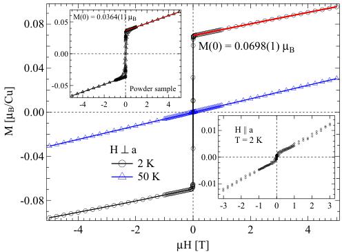
FIG. 4. (Color online) Magnetization as a function of magnetic field was measured on single-crystal \( \alpha-Cu_{2}V_{2}O_{7} \) with \( H \perp a \) at T = 2 and 50 K. The lower inset shows the data for \( H \parallel a \) . The upper inset shows the magnetization as a function of magnetic field measured on a powder sample at T = 5 K.
exchange interaction between \( S_{i} \) and \( S_{j} \) . The DM interaction is present in \( \alpha-Cu_{2}V_{2}O_{7} \) for the Cu1–Cu4 bond [Fig. 1(b)] since there is no inversion center between the magnetic \( Cu^{2+} \) ions [32]. The magnitude of spin canting \( \eta \) resulting from the DM interactions was estimated to be \( \simeq2^{\circ} \) from the previous magnetization measurements on the powder sample [20].
To determine the spin canting and DM parameter on the single-crystal sample, the magnetization measurements as a function of magnetic field up to a maximal field of 5 T were performed with two orthogonal magnetic field orientations, i.e., \( H\|a \) and \( H\perp a \) . Figure 4 shows the magnetization measurement on the single crystal with the applied magnetic field perpendicular to the a axis. Above \( T_{N} \) (T = 50 K) the magnetization is linear throughout the measuring field range. However, below \( T_{N} \) (T = 2 K) starting from zero applied field the magnetization sharply rises to a finite value with only a slight increase in magnetic field before attaining the same linear response as that observed in the 50 K data. The rapid increase of the magnetization, which is indicative of weak ferromagnetism due to the spin canting, is not observed for \( H\|a \) as shown in the lower inset. The small kink around zero field is most likely due to slight misalignment. The same measurements on the power sample show a similar weak ferromagnetic component as shown in the upper inset. However, the jump is less sharp and about a factor of 2 smaller due to powder average. For the single-crystal data, a hysteresis loop, which is typical for ferromagnetism, is not clear with a very small coercive field (<10 Oe, which is the resolution of the measurements), but it is more pronounced for the powder data, possibly due to the powder average over all orientations, which could broaden the magnetization reversal.
Quantitatively, the red line in Fig. 4 (and in the upper inset for the powder sample) denotes a linear fit to the magnetization for \( H \geqslant 5000 \) Oe and is extrapolated to intercept the y axis to obtain the value of \( M(0) \) , the canted moment at zero field.
From the single-crystal (powder) data, \( M(0) = 0.0698(1) \mu_{B} \) [0.0364(1) \( \mu_{B} \) ] is obtained. On the other hand, with \( H \parallel a \) the value of \( M(0) \) is approaching zero as expected since the predominant spin component is antiparallel along the a axis and the canted moments only stay within the bc plane. We note that there exist two sets of the zigzag chains along [011] and [01 \( \bar{1} \) ] on the alternating planes. These chains are about \( 75^{\circ} \) with respect to each other [Fig. 9(b)]. We will assume that for the single-crystal data the measured canted moment \( M(0) \) is a saturated value, where the canted moments on both sets of the chains are aligned along the direction of the applied magnetic field. The canting angle can be calculated from the relation \( \eta = \sin^{-1}\left(\frac{M(0)}{g\mu_{B}S}\right) \) . Given the expected spin-only \( S = \frac{1}{2} \) , g = 2, and \( M(0) \) from the single-crystal data, the canted moment of \( \eta = 4.0^{\circ} \) is obtained.
The direction of the DM vector \( D_{ij} \) is determined by \( r_{\perp} \times r_{ij} \) , where \( r_{ij} \) is a unit vector connecting the spins \( S_{i} \) and \( S_{j} \) , and \( r_{\perp} \) is perpendicular to \( r_{ij} \) and points toward the oxygen ligand as shown in Fig. 1(b). The two pathways Cu1–O(2)–Cu4 and Cu1–O(3)–Cu4 are structurally inequivalent giving rise to noncompensating DM interactions. We note that the DM interactions arising from the two equivalent Cu1–O(1)–Cu2 bonds [Fig. 1(c)] compensate each other resulting in the vanishing DM vector. Although the resulting \( r_{\perp} \times r_{ij} \) does not restrict the DM vector to a specified high-symmetry plane, the cross product of a spin pair, \( S_{i} \times S_{j} \) , constrains the relevant component of the DM vector, which causes the canting, to be only within the bc plane. We will later show in Sec. III C that the canted moments in the bc plane are parallel, and hence the component of \( S_{i} \times S_{j} \) along the a axis vanishes. If only the relevant interaction \( J_{1} \) between Cu1 and Cu4 is taken into account, the in-plane DM parameter \( D_{p} \) can be related to the canting angle \( \eta \) and \( J_{1} \) through the following relation:
\[ \tan(2\eta)=\left|\frac{D_{p}}{J_{1}}\right|, \quad (2) \]
where the absolute value denotes the undetermined direction of the in-plane DM vector.
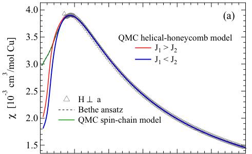
In order to estimate the exchange couplings \( J_{1} \) and \( J_{2} \) , we first analyze magnetic susceptibility based on a weakly coupled spin-chain model ( \( J_{2} \ll J_{1} \) ). We reconsider the magnetic susceptibility as a function of temperature shown in Fig. 3 and fit the data to the result of the high-accuracy numerical Bethe ansatz calculations [33] \( \chi_{\mathrm{Bethe}}(T) \) for the 1D Heisenberg antiferromagnetic system. A fit of the measured magnetic susceptibility (Fig. 5) to
\[ \chi(T)=\chi_{0}+\chi_{\mathrm{B e t h e}}(T), \quad (3) \]
where \( \chi_{0} \) is a temperature-independent susceptibility background, yields \( \chi_{0}=1.68(7)\times10^{-4} \) cm \( ^{3} \) /mol Cu, the intrachain coupling \( J_{1}=5.95(2) \) meV, and the Landé g factor \( g=2.16(1) \) . The Curie-Weiss exchange coupling \( J_{CW}=12.6 \) meV obtained from the mean-field approximation for a number of coordinate spins z=2 is substantially larger than \( J_{1} \) obtained from the susceptibility fit to the spin-chain model ( \( |J_{1}-J_{CW}|/J_{CW}\simeq0.53 \) ) suggesting that the coordination number must be greater than two. Therefore, the interchain interaction is non-negligible. Using Schulz's calculation of the interchain interaction for parallel chains in the mean-field


FIG. 5. (Color online) (a) Fit of magnetic susceptibility with \( H \perp a \) to the Bethe ansatz numerical result (black-dashed line), QMC simulations on the uniform spin-chain model (green line), QMC simulations on the helical-honeycomb model with \( J_{1} > J_{2} \) (red), and with \( J_{1} < J_{2} \) (blue). (b) Residual curves \( (\chi_{\mathrm{data}} - \chi_{\mathrm{fit}}) \) between the data and fit curves of different lattice models.
approximation, \( |J_{inter}| = |J_{2}| = T_{N}/[1.28\sqrt{\ln(5.8J_{intra}/T_{N})}] \) [34], where \( J_{intra} \) is an intrachain interaction, and applying it to \( \alpha-Cu_{2}V_{2}O_{7} \) with \( T_{N} = 33.4 \) K and \( J_{intra} = J_{1} = 5.95 \) meV, we obtain \( |J_{2}| \simeq 1.42 \) meV. Even though the sign of \( J_{2} \) cannot be determined from this calculation, the discrepancy between \( J_{CW} \) for z = 2 and \( J_{1} \) suggests that the interchain interaction is dominantly antiferromagnetic and hence \( J_{2} > 0 \) . Neutron diffraction, which will be discussed in the next section, reveals antiferromagnetic alignment of spins in the [011] and [01 \( \bar{1} \) ] chains on different bc planes as shown in Fig. 9. Therefore, the leading antiferromagnetic interchain interactions [denoted by green bonds in Fig. 9(a)], which induce the antiparallel arrangement of spins along the a axis, link the chains on the adjacent planes giving rise to the helical-honeycomb spin network. The Cu–O–Cu bond angle of this interchain interaction, which is greater than \( 90^{\circ} \) [Fig. 1(c)], is also consistent with the antiferromagnetic coupling. The coupling between the parallel chains in the same bc plane is expected to be much smaller because the bonding is not of the Cu–O–Cu type but must be via the \( V_{2}O_{7} \) double tetrahedra. The value of \( |J_{2}/J_{1}| \simeq 0.23 \) is substantially larger than that measured in other 1D systems such as \( KCuF_{3} \) , \( Sr_{2}CuO_{3} \) , and \( BaCu_{2}Si_{2}O_{7} \) , where the value of \( |J_{inter}/J_{intra}| \) is 0.001–0.01 [35–37], suggesting that the magnetism in \( \alpha-Cu_{2}V_{2}O_{7} \) is far from being an ideal realization of the 1D spin system, and probably invalidating the above analysis.
as well as other previous studies, which are based on the coupled spin-chain model [20,22,23]. Furthermore, we note that since the dominating interchain interaction is between the [011] and [01I] chains, of which the spin coordination number is different from that of the parallel chains, Schulz's results used above could potentially provide an erroneous magnitude of \( J_{2} \) .
To obtain the better estimates of \( J_{1} \) and \( J_{2} \) , we perform QMC simulations with the LOOP algorithm on the helical-honeycomb spin network, which shows a disconnected hexagon when viewed along the b axis [Figs. 9(a) and 9(c)]. The magnetic susceptibility was computed and fit to the data. In addition, the susceptibility for the uniform spin-chain model was calculated and compared with \( \chi_{\mathrm{Bethe}}(T) \) [Eq. (3)]. The QMC numerical results were first fit using the following formula:
\[ \chi^{*}(t)=\frac{1}{4t}\mathcal{P}_{(r)}^{(q)}(t), \quad (4) \]
where \( t = k_{B} T / J_{max} \) and the Padé approximant is given by
\[ \mathcal{P}_{(r)}^{(q)}(t)=\frac{1+\sum_{n=1}^{q}N_{n}/t^{n}}{1+\sum_{n=1}^{r}D_{n}/t^{n}}. \quad (5) \]
The coefficient 1/4 is from \( S(S+1)/3 \) for \( S=\frac{1}{2} \) and the factor 1/t ensures that \( \chi^{*}(t) \) approaches the Curie law at high temperature. \( J_{max} \) is the maximum of \( J_{1} \) and \( J_{2} \) and the smaller interaction is equal to \( \alpha J_{max} \) , where the parameter \( \alpha \) is fixed for each QMC simulation. The numerical parameters \( N_{n} \) and \( D_{n} \) were obtained up to q = 5 and r = 6 from the fit. The resulting Padé approximant for each QMC calculation was then used to fit the measured susceptibility data using
\[ \chi(T)=\chi_{0}+\chi_{\mathrm{Q M C}}(T), \quad (6) \]
where
\[ \chi_{\mathrm{Q M C}}(T)=\frac{N_{A}\mu_{B}^{2}g^{2}}{k_{B}J_{\max}}\chi^{*}(k_{B}T/J_{\max}), \quad (7) \]
to obtain \( J_{max} \) and g. \( N_{A} \) , \( \mu_{B} \) , and \( k_{B} \) are the Avogadro constant, the Bohr magneton, and the Boltzmann constant, respectively. For the helical-honeycomb model, \( \alpha \) is manually adjusted until the best fit is acquired. Figure 5 shows the best fits for both uniform spin-chain and helical-honeycomb models where the obtained fit parameters are summarized in Table II for comparison. The QMC simulation on the spin-chain model exactly match the result obtained from the Bethe ansatz calculations with the same magnitude of \( J_{1} \) , proving the validity to the QMC simulations. For the helical-honeycomb model, two sets of the exchange parameters, for \( J_{1} > J_{2} J_{\max} = 5.79(1) \) meV, \( \alpha = 0.45 \) , and g = 2.24(1) and for \( J_{1} < J_{2} J_{\max} = 6.31(1) \) meV, \( \alpha = 0.65 \) , and g = 2.25(1), fit the data equally well and provide a noticeably better fit than the spin-chain model for most of the temperature range from 300 K down to \( \sim T_{N} \) as shown by the residual analysis in Fig. 5(b). The obtained average exchange interaction \( \bar{J} = (2J_{1} + J_{2})/3 \) for the coupled spin-chain model is much lower than the mean-field value \( J_{CW} \) obtained from the Curie-Weiss fit with \( |\bar{J} - J_{CW}|/J_{CW} \simeq 0.47 \) . Our proposed helical-honeycomb model shows a slightly smaller deviation with \( |\bar{J} - J_{CW}|/J_{CW} \cong 0.44 \) and \( \simeq 0.42 \) for \( J_{1} > J_{2} \) and \( J_{1} < J_{2} \) , respectively. Additional exchange and anisotropic interactions could affect the value of \( \bar{J} \) , potentially leading to closer agreement between \( \bar{J} \) and \( J_{CW} \) . Unfortunately, based on combined susceptibility analysis and QMC simulations, we were unable to uniquely identify the leading coupling constant. It was previously proposed that the leading coupling connects Cu1 and Cu4 via \( J_{1} \) forming the zigzag chains along [011] and [011] directions [Fig. 1(a)], but the competition between ferromagnetic coupling via Cu1–O(3)–Cu4 with the bond angle close to \( 90^{\circ} \) and antiferromagnetic coupling via Cu1–O(2)–Cu4 with the bond angle of \( 106^{\circ} \) [Fig. 1(b)] could render a weaker net antiferromagnetic interaction for \( J_{1} \) than the noncompeting antiferromagnetic coupling \( J_{2} \) between Cu1 and Cu2 via two equivalent Cu1–O(1)–Cu2 bridges [Fig. 1(c)]. Further theoretical analyses based on first-principle calculations, which will provide complementary support to our analysis, are desirable in order to identify the leading interaction.
Given \( J_{1} \) obtained from the two helical-honeycomb models discussed above and the canting angle \( \eta = 4.0^{\circ} \) from the magnetization data, we estimate the in-plane DM parameter \( |D_{p}| \) using Eq. (2) to be 0.814(1) meV for the helical-honeycomb model with \( J_{1} > J_{2} \) and 0.576(1) meV for \( J_{1} < J_{2} \) , or \( \simeq 0.14 J_{1} \) . The values of \( |D_{p}| \) for all considered lattice models are summarized in Table II. The magnitude of the DM vector shows good agreement with Moriya's calculation [32] as \( \Delta g / g \sim 0.12 \sim |D_{p} / J_{1}| \) , where g is the free electron Landé g factor and \( \Delta g \) denotes its shift caused by the crystalline environment. The helical-honeycomb lattice formed by \( J_{1} \) and \( J_{2} \) of comparable strength and the presence of the DM interactions in \( \alpha - Cu_{2} V_{2} O_{7} \) induce the magnetically ordered state below the Néel temperature. Hence, the long-range order observed in this system does not defy the Mermin-Wagner theorem [38].
TABLE II. Parameters obtained from the fit of magnetic susceptibility with \(H \perp a\) using different lattice models.
| Bethe ansatz | QMC (this work) | |||
| Uniform spin chain | Helical-honeycomb | |||
| calculation [33] (coupled spin chain) | \( J_{1} > J_{2} \) | \( J_{1} < J_{2} \) | ||
| \( J_{1} \) (meV) | 5.95(2) | 5.95(2) | 5.79(1) | 4.10(1) |
| \( J_{2} \) (meV) | \( \simeq \) 1.42 | - | 2.61(1) | 6.31(1) |
| g | 2.16(1) | 2.16(1) | 2.24(1) | 2.25(1) |
| \( \chi_{0}(10^{-4} \text{ cm}^{3}/\text{mol Cu}) \) | 1.68(7) | 1.69(7) | 0.94(6) | 0.89(3) |
| \( |D_{p}| \) (meV) | 0.836(3) | 0.836(3) | 0.814(1) | 0.576(1) |


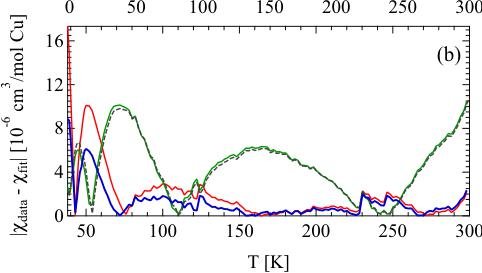
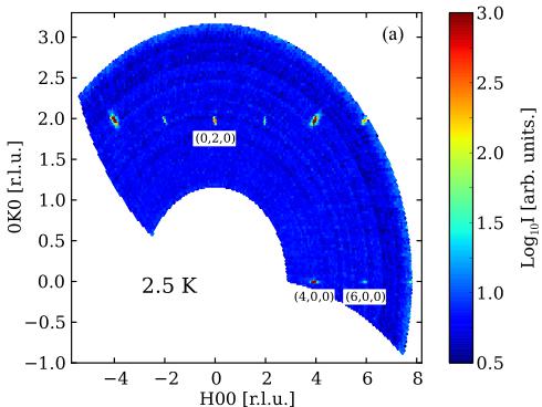
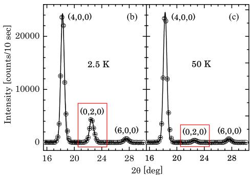
FIG. 6. (Color online) (a) An intensity map of single-crystal \( \alpha \) -Cu \( _{2} \) V \( _{2} \) O \( _{7} \) was measured in the \( (h,k,0) \) plane at 2.5 K. The intensity is presented in a log scale. (b) and (c) show the \( \theta \) -2 \( \theta \) scans around the \( (4,0,0) \) , \( (0,2,0) \) , and \( (6,0,0) \) Bragg reflections at 2.5 and 50 K, respectively. The solid line is a guide to the eye. Error bars represent one standard deviation throughout the article.
C. Neutron diffraction
In order to investigate the magnetic structure of the ordered state, we performed elastic neutron scattering to search for magnetic Bragg reflections. Figures 6(b) and 6(c) show clear extra scattering intensity below \( T_{N} \) at (0,2,0), indicative of magnetic scattering; small peaks at (0,2,0) and (6,0,0), which are structurally forbidden by symmetry, at 50 K are due to higher-order neutron contamination. On the other hand, the intensities at (4,0,0) and (6,0,0), which are also allowed magnetic Bragg reflections, do not show a significant change below \( T_{N} \) . In neutron scattering, only the spin component that is perpendicular to the momentum transfer contributes to the magnetic scattering intensity, due to the dipole-dipole interaction as described by the geometric factor \( \sum_{\alpha,\beta}(\delta_{\alpha,\beta}-\hat{Q}_{\alpha}\hat{Q}_{\beta}) \) [39], where \( \alpha \) denotes the spin components and \( \hat{Q}_{\alpha} \) is the unit vector of Q along the component \( \alpha \) . For \( \alpha \) -Cu \( _{2} \) V \( _{2} \) O\( _{7} \) most of the spin component is parallel to the a axis, which is also evidenced by the magnetic susceptibility. Hence the magnetic Bragg reflections \( (h,0,0) \) become negligibly small.


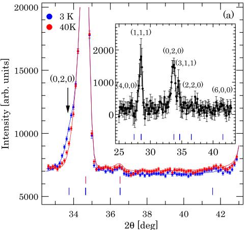
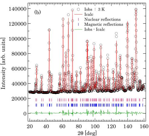
FIG. 7. (Color online) (a) Neutron diffraction data of powder \( \alpha \) -Cu \( _{2} \) V \( _{2} \) O_{7} at 3 K show the magnetic Bragg scattering at (0,2,0) (indicated by an arrow). The inset shows the intensity difference with allowed magnetic Bragg reflections indexed. (b) The powder neutron diffraction data collected at 3 K are refined using FullProf.
The integrated intensity of the \( (0,2,0) \) magnetic Bragg reflection as a function of temperature (Fig. 3 inset) shows an upturn around 33 K indicating a transition to the antiferromagnetic ordered state, coincident with the jump in the magnetic susceptibility [Fig. 3(a)]. A fit of the order parameter to the power law \( I(T) \propto (1 - T/T_{N})^{2\beta} \) for \( 24 < T < 34 \) K gives a critical exponent \( \beta = 0.21(1) \) and \( T_{N} = 33.4(1) \) K. The fit value of \( \beta \) is typical for low-dimensional magnetic systems [35,36,40].
Figure 7 shows the powder neutron diffraction data collected at 3 and 40 K at Echidna to investigate intensity difference due to magnetic scattering. Figure 7(a) shows a small shoulder peak for the 3 K data as indicated by the arrow,
TABLE III. Magnetic representations and their basis vectors for Cu1(x,y,z), Cu2(-x,-y,z), Cu3(x+1/4,-y+1/4,z+1/4), and Cu4(-x+1/4,y+1/4,z+1/4) (see Fig. 1).
| IR | BV | Cu1 | Cu2 | Cu3 | Cu4 | ||||||||
| \( m_{a} \) | \( m_{b} \) | \( m_{c} \) | \( m_{a} \) | \( m_{b} \) | \( m_{\mathrm{c}} \) | \( m_{a} \) | \( m_{b} \) | \( m_{\mathrm{c}} \) | \( m_{a} \) | \(m_{b} \) | \( m_{\mathrm{c}} \) | ||
| \( \Gamma_{1} \) | \( \psi_{1} \) | 1 | 0 | 0 | -1 | 0 | 0 | 1 | 0 | 0 | -1 | 0 | 0. |
| \( \psi_{2} \) | 0 | 1 | 0 | 0 | -1 | 0. | 0 | -1 | 0 | 0 | 1 | 0. | |
| \( \psi_{3} \) | 0 | 0 | 1 | 0 | 0 | 1 | 0 | 0 | 1 | 0 | 0 | 1 | |
| \( \Gamma_{2} \) | \( \psi_{1} \) | 1 | 0 | 1 | 0 | -1 | 0 | 0 | -1 | 0 | 0 | 0 | |
| \( \psi_{2} \) | 0 | 1 | 1 | 0 | 0 | -1 | 0 | 1 | 0 | 0 | -1 | 0, | |
| \( \psi_{3} \) | 0 | 0 | 0 | 1 | 0 | 0 | 1 | ||||||
| \( \Gamma_{3} \) | \( \psi_{1} \) | 1 | 0 | 2 | 0 | 1 | 0 | 0 | 1 | 0 | 0 | -1 | 0 |
| \( \psi_{2} \) | 0 | 1 | 0 | 1 | 0 | 0 | -1 | 0 | -1 | 0 | |||
| \( \psi_{3} \) | 0 | 0 | -1 | 0 | 0 | -1 | 1 | 0 | 0 | ||||
| \( \Gamma_{4} \) | \( \psi_{1} \) | 1 | 0 | 3 | 0 | 1 | 0 | 0 | -1 | 0 | 0 | -1 | 0 |
| \( \psi_{2} \) | 0 | 1 | 4 | 0 | 1 | 0 | 0 | 1 | 0 | ||||
| \( \psi_{3} \) | 0 | 0 | 1 | 0 | 0 | 0 | -1 | 0 | 0 | 1 | 0 | 0 | |
which corresponds to the \( (0,2,0) \) magnetic Bragg reflection. In the inset, the intensity difference between 3 and 40 K data clearly shows the magnetic Bragg reflections at \( (1,1,1) \) , \( (0,2,0) \) , and \( (3,1,1) \) , and negligible magnetic scattering intensities at \( (4,0,0) \) and \( (6,0,0) \) . This absence of magnetic Bragg intensity at the \( (h,0,0) \) reflections is consistent with the single-crystal data discussed previously.
The magnetic structure of \( \alpha-Cu_{2}V_{2}O_{7} \) was analyzed by the irreducible representation theory. The calculations were carried out using the software BasIreps [24]. The decomposition of the irreducible representations (IRs) for \( Cu^{2+} \) ions (16b) can be described by
\[ \Gamma=3\Gamma_{1}+3\Gamma_{2}+3\Gamma_{3}+3\Gamma_{4}. \quad (8) \]
The basis vectors for each IR are summarized in Table III. The coupled intrachain \( Cu^{2+} \) spins are between \( Cu1-Cu4 \) along [011], and between \( Cu2-Cu3 \) along [011]. As discussed above, the antiferromagnetic spin component of the \( Cu^{2+} \) ions is predominantly along the a axis. Therefore, among the four possible magnetic models we can simply rule out \( \Gamma_{2} \) and \( \Gamma_{3} \) , which according to the Bertaut's notation [41] give rise to the \( A_{x} \) and \( F_{x} \) configurations, respectively; both IRs give ferromagnetic spin component along the a axis. On the other hand, \( \Gamma_{1} \) and \( \Gamma_{4} \) , which give rise to the \( G_{x} \) and \( C_{x} \) configurations, respectively, result in the antiferromagnetic arrangement along the a axis for the spins along the zigzag chains. The canted moments, which are in the bc plane, of the spins in the same chain for \( \Gamma_{1} \) and \( \Gamma_{4} \) are parallel. Hence the cross product \( S_{i} \times S_{j} \) does not have a component along the a axis, making the DM component along the a axis irrelevant as previously stated. Both \( \Gamma_{1} \) and \( \Gamma_{4} \) can give rise to the weak ferromagnetism observed in the magnetic susceptibility. However, \( \Gamma_{1} \) gives a better fit to the powder neutron diffraction data. Figure 7(b) shows the full pattern refinements for \( \Gamma_{1} \) with the spin component along the a axis \( m_{x} \) as the only fit parameter while the other two components, i.e., \( m_{y} \) and \( m_{z} \) , were fixed to zero. The magnetic R factors from the refinements for \( \Gamma_{1} \) and \( \Gamma_{4} \) , yield 0.040 and 0.134, respectively, attesting to the validity of \( \Gamma_{1} \) over \( \Gamma_{4} \) . The obtained magnetic moment along the a axis \( m_{x} \) is \( 0.9(2) \) \( \mu_{B} \) for \( \Gamma_{1} \) .

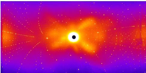
FIG. 8. (Color online) False color representation of the single-crystal neutron diffraction measured at 4 K on the Laue diffractometer Koala. The halo around the center of the image is due to scattering from a polycrystalline aluminum crystal holder.
To further confirm the magnetic structure and obtain a better estimate of the ordered moment, we performed single-crystal neutron diffraction at the Laue diffractometer, Koala. The diffraction data were collected at 4 and 50 K to investigate the nuclear and magnetic structure. The Laue diffraction pattern measured at 4 K shows distinct Bragg peaks (Fig. 8). The structural parameters for the 50 K data were refined against \( Fdd2 \) space group using \( ShelXle \) yielding \( R_{1}=0.081 \) for 998 reflections with \( F_{obs}<4\sigma(F_{obs}) \) . The result is in agreement with the single-crystal x-ray diffraction refinement (see Table I). For the 4 K data, where the system becomes magnetically ordered, the magnetic structure refinements were performed using Jana2006 [42]. The reflections were refined against Shubnikov space group \( Fd'd'2 \) , which is equivalent to the irreducible representation \( \Gamma_{1} \) that gives the best fit to the magnetic structure in this system. The spin components along the b and c axes were fixed to zero due to the unresolved spin canting. The ordered moment along the a axis \( m_{x}=0.93(9)\mu_{B} \) was obtained with wR=0.051. This value of the ordered moment, which is consistent with the value obtained from powder neutron diffraction, is slightly lower than (but close to) the expected value of \( 1\mu_{B} \) . This discrepancy could be a result from the constrained spin component to only the a axis, discarding the spin canting that is not obtainable from the neutron diffraction data. In addition, quantum fluctuations might also play a role in reducing the ordered moment. The antiferromagnetic spin structure on the helical-honeycomb lattice is depicted in Fig. 9(a). The spins on the parallel zigzag chains ferromagnetically align as a result of the antiferromagnetic coupling \( J_{2} \) around the helical-honeycomb loop as shown in Fig. 9(c), allowing the ordering to propagate along the transverse directions and prompting the 3D long-range order. Due to the very small spin canting we cannot determine the magnitude and direction of the canted moments in the bc plane from the neutron diffraction data. However, \( \Gamma_{1} \) allows the canted moments of the spins on the same chain to be parallel. For the spins on the different chains that are located on the adjacent bc plane, the c component (b component) is parallel (antiparallel) as shown in Fig. 9(b).

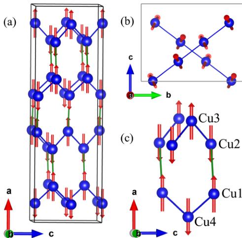
FIG. 9. (Color online) (a) The magnetic structure of the \( S=\frac{1}{2}Cu^{2+} \) spins in \( \alpha-Cu_{2}V_{2}O_{7} \) shows the major spin component along the a axis with the antiferromagnetic arrangement. Blue bonds represent \( J_{1} \) while green bonds \( J_{2} \) . (b) The two zigzag chains connected by \( J_{1} \) ( \( J_{2} \) not shown) on adjacent bc planes are along [011] and [01 \( \bar{1} \) ] and are about \( 75^{\circ} \) with respect to each other. We note that the canted moments in the bc plane are exaggerated for visualization, and the drawn spins do not represent the actual canting, neither in terms of magnitude nor direction. (c) The connectivity of \( J_{1} \) and \( J_{2} \) gives rise to the helical-honeycomb pattern when viewed along the b axis.
IV. SUMMARY
We have proposed a spin model to describe magnetic properties of \( \alpha-Cu_{2}V_{2}O_{7} \) . Combined studies of magnetization, QMC simulations, and neutron diffraction show the helical-honeycomb pattern of spin network connected by two different exchange couplings. Magnetic susceptibility shows a broad peak at \( \sim50 \) K, which is an evidence of rising short-range spin correlations, followed by an abrupt increase indicative of a phase transition to a magnetically ordered state at \( T_{N}=33.4(1) \) K. The Bethe ansatz calculations for the \( S=\frac{1}{2} \) uniform Heisenberg chain fit the \( H\perp a \) data very well above \( T_{N} \) but our proposed helical-honeycomb model shows substantial improvement of the fit for \( J_{1}:J_{2}=1:0.45 \) with \( J_{1}=5.79(1) \) meV and for \( J_{1}:J_{2}=0.65:1 \) with \( J_{2}=6.31(1) \) meV. Therefore, we conclude that the helical-honeycomb model describes the underlying spin network of \( \alpha-Cu_{2}V_{2}O_{7} \) more accurately than the previously held spin-chain model.
[1] J. C. Bonner and M. E. Fisher, Phys. Rev. 135, A640 (1964).
[2] S. Sachdev, Nat. Phys. 4, 173 (2008).
[3] H. Bethe, Z. Phys. 71, 205 (1931).
[4] M. Hase, I. Terasaki, and K. Uchinokura, Phys. Rev. Lett. 70, 3651 (1993).
[5] J. Riera and A. Dobry, Phys. Rev. B 51, 16098 (1995).
The anisotropy below \( T_{N} \) suggests that the majority of the spin component is along the crystallographic a axis, which is confirmed by neutron diffraction experiments. The weak ferromagnetism is a result of spin canting within the bc plane due to the DM interactions. Magnetization measurements with \( H \perp a \) show the spontaneous magnetization from which the canting angle \( \eta \) of \( 4.0^{\circ} \) and the in-plane DM parameter \( |D_{p}| \simeq 0.14J_{1} \) are obtained.
The analysis of the neutron diffraction data shows that the \( S=\frac{1}{2} \) Cu \( ^{2+} \) spins antiferromagnetically align along the helical-honeycomb loops with the ordered moment of 0.93(9) \( \mu_{B} \) predominantly along the crystallographic a axis. The spin network of two comparable exchange couplings forming the helical-honeycomb lattice and the DM interactions lead to the long-range magnetic ordering below \( T_{N} \) . However, due to the complex exchange pathways and the presence of weak frustration, the exact value of both exchange interactions could deviate from our analysis. Further theoretical analyses based on first-principle calculations and studies of spin dynamics by means of inelastic neutron scattering are therefore required in order to better determine the exchange interactions and confirm the helical-honeycomb spin model. With the current availability of large single crystals, an inelastic neutron scattering study is possible and will reveal a complete picture of the relevant microscopic Hamiltonian parameters, as well as influences of the low spin-coordination number and quantum fluctuations on spin dynamics.
Note added in proof. Recently, we became aware of the work by Sannigrahi et al. [43], in which they performed density functional theory to calculate the relevant exchange interactions in \( \alpha-Cu_{2}V_{2}O_{7} \) . However, the QMC calculations of the susceptibility show that their lattice model with the dominant third-nearest-neighbor antiferromagnetic interactions ( \( J_{3}=13.61~meV \) ) gives a broad peak at a higher temperature than \( \sim50~K \) , inconsistent with the experimental data.
ACKNOWLEDGMENTS
Work at Mahidol University was in part supported by the Thailand Research Fund Grant No. MRG5580022 and the Thailand Center of Excellence in Physics. Work at IMRAM was partly supported by Japan Society for the Promotion of Science KAKENHI Grant No. 24224009. The authors, G.G. and K.M., would like to thank I. M. Tang and T. Osotchan for the use of their laboratory equipment and M. A. Allen for useful discussions. The identification of any commercial product or trade name does not imply endorsement or recommendation by the National Institute of Standards and Technology.
[6] M. Shaz, S. van Smaalen, L. Palatinus, M. Hoinkis, M. Klemm, S. Horn, and R. Claessen, Phys. Rev. B 71, 100405(R) (2005).
[7] E. T. Abel, K. Matan, F. C. Chou, E. D. Isaacs, D. E. Moncton, H. Sinn, A. Alatas, and Y. S. Lee, Phys. Rev. B 76, 214304 (2007).
[8] A. W. Garrett, S. E. Nagler, D. A. Tennant, B. C. Sales, and T. Barnes, Phys. Rev. Lett. 79, 745 (1997).
[9] M. Mourigal, M. Enderle, A. Klöpperpieper, J. S. Caux, A. Stunault, and H. M. Rønnow, Nat. Phys. 9, 435 (2013).
[10] T. Nikuni, M. Oshikawa, A. Oosawa, and H. Tanaka, Phys. Rev. Lett. 84, 5868 (2000).
[11] J. des Cloizeaux and J. J. Pearson, Phys. Rev. 128, 2131 (1962).
[12] Y. Endoh, G. Shirane, R. Birgeneau, P. Richards, and S. Holt, Phys. Rev. Lett. 32, 170 (1974).
[13] K. Momma and F. Izumi, J. Appl. Crystallogr. 44, 1272 (2011).
[14] G. M. Clark and R. Garlick, J. Inorg. Nucl. Chem. 40, 1347 (1978).
[15] S. V. Krivovichev, S. K. Filatov, P. N. Cherepansky, T. Armbruster, and O. Y. Pankratova, Can. Mineral. 43, 671 (2005).
[16] T. I. Krasnenko, M. V. Rotermel, S. A. Petrova, R. G. Zakharov, O. V. Sivtsova, and A. N. Chvanova, Russ. J. Inorg. Chem. 53, 1641 (2008).
[17] C. Calvo and R. Faggiani, Acta Crystallogr. Sect. B 31, 603 (1975).
[18] P.D. Robinson, J.M. Hughes, and M. I. Malinconico, American Mineralogist 72, 397 (1987).
[19] J. B. Goodenough, Phys. Rev. 100, 564 (1955); J. Kanamori, J. Phys. Chem. Solids 10, 87 (1959); P. W. Anderson, Solid State Phys. 14, 99 (1963).
[20] J. Pommer, V. Kataev, K.-Y. Choi, P. Lemmens, A. Ionescu, Y. Pashkevich, A. Freimuth, and G. Güntherodt, Phys. Rev. B 67, 214410 (2003).
[21] A. A. Tsirlin, O. Janson, and H. Rosner, Phys. Rev. B 82, 144416 (2010).
[22] L. A. Ponomarenko, A. N. Vasil'ev, E. V. Antipov, and Y. A. Velikodny, Physica B 284-288, 1459 (2000).
[23] M. Touaiher, K. Rissouli, K. Benkhouja, M. Taibi, J. Aride, A. Boukhari, and B. Heulin, Mater. Chem. Phys. 85, 41 (2004).
[24] J. Rodriguez-Carvajal, Physica B 192, 55 (1993).
[25] C. B. Hübschle, G. M. Sheldrick, and B. Dittrich, J. Appl. Crystallogr. 44, 1281 (2011).
[26] S. Todo and K. Kato, Phys. Rev. Lett. 87, 047203 (2001); H. G. Evertz, Adv. Phys. 52, 1 (2003).
[27] A. Albuquerque, F. Alet, P. Corboz, P. Dayal, A. Feiguin, S. Fuchs, L. Gamper, E. Gull, S. Gürtler, A. Honecker, R. Igarashi, M. Körner, A. Kozhevnikov, A. Läuchli, S. R. Manmana, M.
Matsumoto, I. P. McCulloch, F. Michel, R. M. Noack, G. Pawlowski, L. Pollet, T. Pruschke, U. Schollwöck, S. Todo, S. Trebst, M. Troyer, P. Werner, and S. Wessel, J. Magn. Magn. Mater. 310, 1187 (2007).
[28] J. W. Lynn, Y. Chen, S. Chang, Y. Zhao, S. Chi, W. Ratcliff II, B. G. Ueland, and R. W. Erwin, J. Res. Natl. Inst. Stand. Technol. 117, 60 (2012).
[29] R. Piltz, Acta Crystallogr. Sect. A 67, C155 (2011).
[30] H. P. Christian and H. Müller-Buschbaum, Z. Naturforsch. B 29, 713 (1974).
[31] B. V. Slobodin and R. F. Samigullina, Inorg. Mater. 46, 196 (2010).
[32] T. Moriya, Phys. Rev. Lett. 4, 228 (1960).
[33] D. C. Johnston, R. K. Kremer, M. Troyer, X. Wang, A. Klümper, S. L. Bud'ko, A. F. Panchula, and P. C. Canfield, Phys. Rev. B 61, 9558 (2000).
[34] H. J. Schulz, Phys. Rev. Lett. 77, 2790 (1996).
[35] K. M. Kojima, Y. Fudamoto, M. Larkin, G. M. Luke, J. Merlin, B. Nachumi, Y. J. Uemura, N. Motoyama, H. Eisaki, S. Uchida, K. Yamada, Y. Endoh, S. Hosoya, B. J. Sternlieb, and G. Shirane, Phys. Rev. Lett. 78, 1787 (1997).
[36] D. A. Tennant, S. E. Nagler, D. Welz, G. Shirane, and K. Yamada, Phys. Rev. B 52, 13381 (1995).
[37] I. Tsukada, Y. Sasago, K. Uchinokura, A. Zheludev, S. Maslov, G. Shirane, K. Kakurai, and E. Ressouche, Phys. Rev. B 60, 6601 (1999).
[38] N. D. Mermin and H. Wagner, Phys. Rev. Lett. 17, 1133 (1966).
[39] G. Shirane, S. M. Shapiro, and J. M. Tranquada, Neutron Scattering with a Triple-Axis Spectrometer (Cambridge University Press, Cambridge, England, 2002).
[40] M. G. Banks, R. K. Kremer, C. Hoch, A. Simon, B. Ouladdiaf, J. M. Broto, H. Rakoto, C. Lee, and M. H. Whangbo, Phys. Rev. B 80, 024404 (2009).
[41] E. F. Bertaut, Magnetism (Academic, New York, 1963), Vol. 3.
[42] V. Petříček, M. Dušek, and L. Palatinus, Z. Kristallogr. 229, 345 (2014).
[43] J. Sannigrahi, S. Bhowal, S. Giri, S. Majumdar, and I. Dasgupta Phys. Rev. B 91, 220407(R) (2015).
 p2_0.jpg
 p3_0.jpg
 p4_0.jpg
 p4_1.jpg
 p5_0.jpg
 p5_1.jpg
 p7_0.jpg
 p7_1.jpg
 p7_2.jpg
 p7_3.jpg
 p8_0.jpg
 p9_0.jpg