| Transition Temperature | 5.3 K |
|---|---|
| Propagation Vector | k1 (0, 0, 0) |
| Parent Space Group | I4/mcm (#140) |
| Magnetic Space Group | Fm'mm (#69.523) |
| Magnetic Point Group | m'mm (8.3.26) |
| Lattice Parameters | 5.5150 5.5150 7.8050 90.0000 90.0000 90.0000 |
|---|---|
| DOI | 10.1103/physrevb.86.094432 |
| Reference | V. Scagnoli, M. Allieta, H. Walker, M. Scavini, T. Katsufuji, L. Sagarna, O. Zaharko and C. Mazzoli, Physical Review B (2012) 86. |
| Label | Element | Mx | My | Mz | |M| |
|---|---|---|---|---|---|
| Eu1 | Eu | -4.9 | -4.9 | 0.0 | 6.93 |
EuTiO_{3} magnetic structure studied by neutron powder diffraction and resonant x-ray scattering
Valerio Scagnoli, \( ^{1,2,*} \) Mattia Allieta, \( ^{3} \) Helen Walker, \( ^{2,*} \) Marco Scavini, \( ^{5} \) Takuro Katsufuji, \( ^{6} \) Leyre Sagrama, \( ^{7} \) Oksana Zaharko, \( ^{8} \) and Claudio Mazzoli \( ^{2,9} \)
\( ^{1} \) Swiss Light Source, Paul Scherrer Institut, CH 5232 Villigen PSI, Switzerland
\( ^{2} \) European Synchrotron Radiation Facility, BP 220, 38043 Grenoble Cedex 9, France
\( ^{3} \) Dipartimento di Chimica, Università degli Studi di Milano, Via Golgi 19, 20133 Milano, Italy
\( ^{4} \) Deutsches Elektronen-Synchrotron DESY, 22607 Hamburg, Germany
\( ^{5} \) Dipartimento di Chimica, Università degli Studi di Milano, ISTM-CNR and INSTM Unit, Via Golgi 19, 20133 Milano, Italy
\( ^{6} \) Department of Physics, Waseda University, Tokyo 169-8555, Japan
\( ^{7} \) Swiss Federal Laboratories for Materials Sciences and Technology (Empa), Solid State Chemistry and Catalysis, Überlandstrasse 129, 8600 Dübendorf, Switzerland
\( ^{8} \) Laboratory for Neutron Scattering, Paul Scherrer Institut, CH 5232 Villigen PSI, Switzerland
(Received 28 June 2012; revised manuscript received 7 September 2012; published 26 September 2012)
We combine neutron powder diffraction and x-ray single-crystal magnetic diffraction at the Eu \( L_{2} \) edge to scrutinize the magnetic motif of the Eu ions in magnetoelectric \( EuTiO_{3} \) . Our measurements are consistent with an antiferromagnetic G-type pattern with the Eu magnetic moments ordering along the a,b-plane diagonal. Recent reports of a novel transition at 2.75 K with a flop of magnetic moments upon poling the sample in an electric field cannot be confirmed for a nonpoled sample. Our neutron diffraction data do not show any significant change of the structure below the Néel temperature. Magnetolecular coupling, if present, is therefore expected to be negligible.
DOI: 10.1103/PhysRevB.86.094432
PACS number(s): 75.25.-j, 75.47.Lx, 75.85.+t, 61.05.fm
I. INTRODUCTION
Multiferroic materials attract a great deal of interest due to the complex phenomena arising from multiple coupled order parameters existing in the same system. \( ^{1} \) An interesting subfamily are the magnetoelectric multiferroics, where it is possible to control the ferroelectric polarization via a magnetic field \( ^{2} \) and the magnetization by an electric field. \( ^{3} \)
The interplay of spin and other electronic or lattice degrees of freedom can induce giant magnetoelectric effects, \( ^{4,5} \) as well as novel types of excitations, \( ^{6} \) paving the way for future applications in sensors, data storage, and spintronics. \( ^{7,8} \) A material which has recently attracted attention is magnetoelectric \( EuTiO_{3} \) , which show an unusual coupling between dielectric, magnetic, and structural degrees of freedom. It can also be deposited as high quality epitaxial thin films, \( ^{9} \) a prerequisite for envisaging practical application in functional devices. Moreover, the presence of a large polarization and ferromagnetism in strained films has been predicted theoretically and reported experimentally, although only at very low temperatures so far. \( ^{10,11} \)
At room temperature bulk \( EuTiO_{3} \) possesses a cubic crystal structure described by the prototype perovskite \( Pm\bar{3}m \) space group. \( ^{12} \) A structural transition \( ^{13,14} \) to the tetragonal \( I4/mcm \) space group has been recently reported. The transition temperature is still controversial. Specific heat measurements suggest a structural instability at \( T_{A}=282 \) K, \( ^{14} \) while high resolution x-ray powder diffraction is able to resolve a peak splitting due to the cubic to tetragonal transition only at \( T_{B}=235 \) K. \( ^{13} \) In order to reconcile this discrepancy Allieta et al. propose the presence of short-range correlation in the transient regime between \( T_{A} \) and \( T_{B} \) , a position supported by results from their pair distribution function analysis below \( T_{A} \) . \( ^{13} \)
At \( T_{N}=5.3 \) K the localized 4f moments on the \( Eu^{++} \) ( \( S=7/2, L=0 \) ) sites order in a G-type antiferromagnetic arrangement, \( ^{15} \) that is, the six nearest neighbors have opposite spins while the 12 next-nearest neighbors have parallel spins. Concomitant with the onset of antiferromagnetism, the dielectric constant decreases abruptly ( \( \sim3.5\% \) ) and shows a strong enhancement as a function of the applied magnetic field ( \( \sim7\% \) at \( B\sim1.5 \) T), providing evidence for magnetoelectric coupling. \( ^{16,17} \) From the dielectric point of view, \( EuTiO_{3} \) is described as a quantum paraelectric, as its low temperature dielectric constant increases on cooling and saturates below approximately 30 K. \( ^{16} \) No long-range polarization is known to set in, despite high values of susceptibility, typical of a paraelectric state stabilized by quantum fluctuations. \( ^{18} \)
In bulk magnetoelectrics the coupling between various degrees of freedom is realized at a microscopic level, \( ^{19} \) hence a detailed knowledge of the crystallographic and magnetic structure is vital to any further investigation and modeling. Following the recent report of a structural transition, \( ^{13} \) we reexamined the low temperature magnetic structure by the combined use of neutron and x-ray magnetic diffraction. Both techniques have been successfully applied to study the complex magnetic structure of several magnetoelectric multiferroic materials, \( ^{20-25} \) most notably \( TbMnO_{3} \) \( ^{26-30} \) and \( YMn_{2}O_{5} \) . \( ^{31-34} \)
II. EXPERIMENTAL DETAILS
Polycrystalline \( EuTiO_{3} \) powder was prepared by solid-state reaction. A stoichiometric mixture of \( Eu_{2}O_{3} \) (99.9% purity; Metall Rare Earth Limited) and \( TiO_{2} \) (99%–100%; Sigma-Aldrich) was ball-milled and reacted for 10 h at \( 1000\ ^{\circ}C \) under a flowing mixture of 5% \( H_{2} \) in Ar (100 ml/min). The resulting phase purity was checked by laboratory x-ray powder diffraction. Part of the powder was reground and pressed into bars ( \( 13\times2\times2\ mm \) ) using \( 10^{4} \) Pa uniaxial pressure. Finally the
bars were sintered for a further 10 h at 1000 °C under a reducing atmosphere (100 ml/min of 5% \( H_{2} \) in Ar). A small fragment of such a bar (9.6 mg) was used to measure the specific heat and the results were found to be consistent with the literature. \( ^{14} \) Single crystals were grown in a floating-zone furnace. \( ^{35} \) For the low temperature phase we refer always to the tetragonal \( I4/mcm \) crystallographic structure (space group 140 with lattice constants \( a = 5.508 \, \AA \) and \( c = 7.805 \, \AA \) at 80 K).
Neutron powder diffraction experiments were performed at the D2B and D20 beamlines at the Institut Laue Langevin, Grenoble, France. 4.47 g of \( EuTiO_{3} \) powder was put in a 57 mm long double walled vanadium sample holder with 11 mm outer diameter and a 1 mm inner ring space for the sample. The experiments at D20 were performed with a wavelength \( \lambda = 0.8127 \AA \) to minimize the Eu absorption. Acquisition of a single pattern took roughly 2 h. At D2B data collection was performed with a wavelength of 1.594 Å and a high resolution setup. Data acquisition of a single pattern took roughly 12 h and was therefore performed only at 1.5 and 12 K due to time constraints. At both beamlines the neutron flux was of the order of \( 10^{7} \) neutrons/s. Refinements of the powder neutron diffraction data were carried out using the FULLPROF \( ^{36} \) program, with the use of its internal tables for scattering lengths and magnetic form factors. A symmetry analysis was performed using the method of Bertaut \( ^{37} \) as implemented in the BASIREPS \( ^{38} \) program to determine all possible spin configurations that are compatible with the tetragonal symmetry of the compound.
Resonant x-ray scattering experiments were performed on a \( EuTiO_{3} \) single crystal at the \( ID20^{39,40} \) beamline of the European Synchrotron Radiation Facility, Grenoble, France. The x-ray energy was tuned in the vicinity of the Eu \( L_{2} \) edge, at approximately 7.610 keV (corresponding to a wavelength of 1.629 Å). The beamline energy resolution was 1 eV. Vertical and horizontal scattering geometries were used such that the beamline provides \( \sigma \) and \( \pi \) polarized photons, respectively. \( \sigma \) ( \( \pi \) ) polarization is perpendicular (parallel) to the diffraction plane. A gold (222) crystal was used for polarization analysis of the diffracted beam (whose state of polarization is denoted by primed quantities). For \( \pi' \) scattering, the suppression of the \( \sigma' \) channel was approximately 99.9%, and vice versa. Analysis of the polarization of the diffracted intensity enables the estimation of the Stokes parameters \( \mathbf{P} = (P_{1}, P_{2}, P_{3}) \) , which describe the state of the polarization of the diffracted beam. When the polarization is linear, the mean helicity is zero and \( P_{3} = 0 \) . \( P_{1} \) represents the linear polarization parallel ( \( P_{1} = -1 \) ) and perpendicular ( \( P_{1} = 1 \) ) to the scattering plane. \( P_{2} \) represents the linear polarization at plus or minus \( 45^{\circ} \) . We use P to refer to the polarization state of the incident x rays and \( P' \) to refer to the polarization state of the diffracted x rays. \( ^{41} \) The polarization analyzer setup can be rotated around the scattered beam by an angle \( \eta \) . At each point the integrated intensity can be determined by rocking the analyzer's \( \theta \) axis ( \( \theta_{PA} \) ). The resulting integrated intensities can then be fitted to the equation
\[ I=\frac{P_{0}^{\prime}}{2}(1+P_{1}^{\prime}\cos2\eta+P_{2}^{\prime}\sin2\eta) \quad (1) \]
to obtain the Poincaré-Stokes parameters \( P_{1}^{\prime} \) and \( P_{2}^{\prime} \) . \( P_{0}^{\prime} \) is proportional to the intensity of the incident x-ray beam. \( ^{[41-43]} \) The linear polarization of the incident photons can be rotated by the use of diamond phase plates \( ^{[41,43,44]} \) and also circularly polarized light can be produced. \( ^{[45]} \) The \( EuTiO_{3} \) single crystal was cut in order to have the [001] direction (as well as the [110] one, given the presence of crystallographic twins, due to the cubic-tetragonal phase transition) perpendicular to the sample surface. The chosen facet was then mechanically polished with fine diamond powder to have a shiny surface.
III. RESULTS AND DISCUSSION
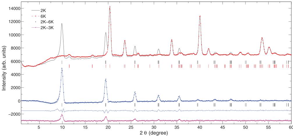
We discuss first the results of our neutron powder diffraction. High resolution data at 12 K were found consistent with the tetragonal structural model proposed in Ref. 13. The \( TiO_{6} \) octahedral tilt angle value obtained at 12 K ( \( \phi = 3.89 \pm 0.06 \) ) follows the temperature evolution suggested by Allieta et al. in Ref. 13. Figure 1 illustrates neutron powder patterns collected above and below the antiferromagnetic ordering temperature, as well as their difference. The magnetic Bragg peaks appear below \( T_{N} \) and can be indexed with a propagation vector \( \mathbf{k} = (0, 0, 0) \) . The Eu ions sit at \( (0, \frac{1}{2}, \frac{1}{4}) \) , which corresponds to the Wyckoff position (4b). There are only two irreducible representations (irreps) associated with the 4b site and the \( (0, 0, 0) \) propagation vector supporting antiferromagnetic ordering: \( \Gamma_{mag} = \Gamma_{6} \oplus \Gamma_{9} \) . \( \Gamma_{6} \) (one-dimensional) supports antiferromagnetic ordering along the c axis while \( \Gamma_{9} \) (bidimensional) favors an antiferro-type order within the a,b plane. It is in general possible to distinguish the a,b plane ordering from the c axis one as neutrons are only sensitive to the magnetic moment component perpendicular to the scattering wave vector. As an example, the absence of the (002) magnetic reflection would suggest the moments to lie along the c axis. Vice versa, the observation of the (002) reflection would support the presence of magnetic ordering in the a,b plane. Unfortunately, the magnetic structure factor in our particular case is zero for both the \( \{001\} \) and the \( \{hk0\} \) reflection families and therefore the selection rules cannot be applied. The two solutions were tested against the data giving similar agreement factors ( \( R_{mag} = 12.4 \) ) and therefore no conclusive statement can be made about the magnetic structure. The value of the \( Eu^{++} \) magnetic moment ( \( \mu = 7 \pm 1 \mu_{B} \) ) was found to be consistent to the free ion as previously reported. \( ^{13} \) The large uncertainty arises from the large neutron cross section of the Eu ions, which severely affects the observed intensities.
Single crystal neutron diffraction would be needed in order to clarify the motif of the Eu magnetic moments, but given the large Eu neutron absorption cross section, we discarded this possibility. In such cases magnetic x-ray diffraction constitutes an appealing alternative to neutron diffraction. The x-ray cross section for magnetic scattering is normally very small. However, at synchrotron photon sources such weak signals are routinely measurable. X-ray magnetic scattering rotates the polarization of the incoming x rays, which may be conveniently studied with the help of a polarizer crystal. The main advantage of using x rays to study magnetism is given by the element sensitivity that is achieved when working close to an atomic absorption edge. Resonant x-ray diffraction occurs when a photon excites a core electron to empty states, and is subsequently reemitted when the electron and the core hole recombine. \( ^{46-48} \) This process introduces

FIG. 1. (Color online) Neutron powder diffraction of \( EuTiO_{3} \) above (red square) and below (black continuous line) \( T_{N} \) (measured on D20, with \( \lambda = 0.8127 \AA \) ). The Rietveld refinement of the difference pattern is plotted with the experimental difference (blue continuous and blue circle, respectively). Bars indicate the position of the magnetic (black) and structural (red) diffraction peaks. The first line below the bars represents the difference between the observed intensities and the one modeled. Finally, we also show the difference between patterns collected at 2 and 3 K (magenta diamond). Data are shifted for clarity.
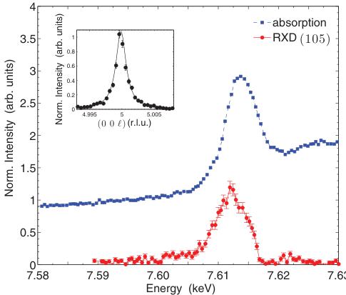
anisotropic contributions to the x-ray susceptibility tensor, \( ^{49-51} \) the amplitude of which increases dramatically as the photon energy is tuned to an atomic absorption edge. In the presence of long-range magnetic order, or a spatially anisotropic electronic distribution, the interference of the anomalous scattering amplitudes may lead to Bragg peaks at positions forbidden by the crystallographic space group. An example of such a resonance enhancement occurring at the Eu \( L_{2} \) edge for the magnetic intensity in \( EuTiO_{3} \) is given in Fig. 2. X rays thus prove to be a valid alternative or complementary tool to neutron diffraction for the study of magnetic structures. \( ^{52,53} \) In addition, its superior resolution in reciprocal space simplifies the precise determination of incommensurate magnetic phases, a worthwhile property in cases where the incommensurability is very small. \( ^{54} \)
We therefore performed a study of the Eu magnetic motif by taking advantage of the resonant enhancement of the magnetic intensities occurring at the Eu \( L_{2} \) edge. At this edge, which corresponds to a 2p to 5d electric dipolar transition, sensitivity to magnetism arises from the hybridization between the 4f and 5d wave functions. The x-ray magnetic cross section depends on the direction of the magnetic moments relative to the polarization of the x rays. This dependence is exploited by rotating the sample about the diffraction wave vector and collecting intensities as a function of the so-called azimuthal angle \( \psi \) . When the azimuthal degree of freedom is not available (e.g., experiments in a magnetic field) or when a sample is prone to have domains, an alternative approach is to keep the sample fixed at a given azimuthal angle and to instead change the direction of the polarization of the incident x rays, the so-called linear polarization scan (or, shortly, polscan). \( ^{41} \) We call \( \zeta \) the angle that materializes this rotation. In our x-ray experiments we have combined both approaches. First, we have performed an experiment with the sample cooled by a helium flow cryostat in horizontal

FIG. 2. (Color online) The (blue) square points represent the x-ray absorption spectrum across the Eu \( L_{2} \) edge recorded in fluorescent mode. The (red) dots represent the intensity of the (105) magnetic reflection (RXD energy scan) in the \( \pi^{\prime}\sigma \) polarization channel. Lines are guide to the eye. The inset shows a reciprocal lattice scan of the diffracted intensity recorded with polarization analysis ( \( \pi^{\prime}\sigma \) ) at the \( L_{2} \) edge corresponding to an incident x-ray energy of 7.612 keV. The magnetic peak has a Lorentzian shape with a full width at half maximum of \( 2.0(1)\times10^{-3} \) r.l.u. Measurements were performed at 2 K.

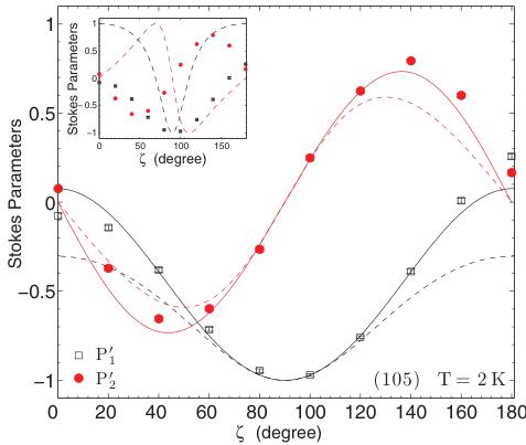
FIG. 3. (Color online) A plot of the measured Poincaré-Stokes parameters \( P_{1}^{\prime} \) (open symbol) and \( P_{2}^{\prime} \) (closed symbol) of the scattered beam as a function of the incident x-ray polarization angle \( \zeta \) of the (105) magnetic reflection. Lines are a simulation according to the magnetic model presented in the main text. The dashed lines simulate \( P_{1}^{\prime} \) (black), and \( P_{2}^{\prime} \) (red) for a sample with equal population of the two \( 90^{\circ} \) domains. The continuous lines represent a fit with the domain population as the only free parameter, indicating that the domains contribute \( 60 \pm 4\% \) and \( 40 \pm 3\% \) of the diffracted intensity, respectively. Measurements were performed in the vicinity of the Eu \( L_{2} \) edge at \( \psi = 0^{\circ} \) , which corresponds to having the a axis in the diffraction plane. The inset shows the simulation of the Poincaré-Stokes parameters expected for a magnetic motif with the moments along the c axis. The measurements were performed at 7.612 keV.
scattering geometry. The diffraction plane was defined by the [001] and the [100] directions. Given the lack of freedom to vary the azimuthal angle, we performed a polscan whose results are shown in Fig. 3. It illustrates the measured values for the Stokes parameters of the (105) magnetic reflection at 2 K. Second, we have complemented such studies with an azimuthal angle dependence of the (341) reflection which is shown in Fig. 4 (performed in vertical scattering geometry with the sample mounted in a closed-cycle He refrigerator). The helium flow cryostat was initially preferred due to its superior temperature stability at the magnetic ordering temperature of \( EuTiO_{3} \) .
Let us discuss our results. To understand the origin of the x-ray resonant magnetic cross section, it is customary to use the expression first derived by Hannon and Trammel for an electric dipole (E1) event: \( ^{46-48} \)
\[ f_{E1,\boldsymbol{\xi}}^{E1}=(\boldsymbol{\epsilon}^{\prime}\cdot\boldsymbol{\epsilon})F^{(0)}-i(\boldsymbol{\epsilon}^{\prime}\times\boldsymbol{\epsilon})\cdot\hat{\boldsymbol{z}}_{n}F^{(1)}, \quad (2) \]
where the first term contributes to the charge Bragg peak. The second term corresponds to magnetic diffraction. \( \hat{z}_{n} \) is a unit vector in the direction of the magnetic moment of the nth ion in the unit cell, and \( \epsilon \) ( \( \epsilon' \) ) describes the polarization state on the incoming (outgoing) x rays. \( ^{55} \) It is then clear that the intensity of the magnetic diffraction depends on the motif of the magnetic moments and therefore on the orientation of the sample relative to the incident x-ray polarization state. In particular a noncollinear magnetic motif will produce

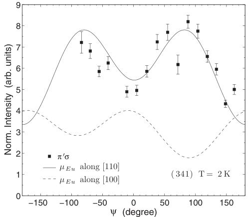
FIG. 4. Azimuthal angle dependence of the (341) magnetic reflection. The continuous line represents a fit to the data with the magnetic moments along the [110] direction. The dotted line a fit with the moments along the [100] direction. Measurements were performed in the vicinity of the Eu \( L_{2} \) edge. The azimuthal angle equals zero when the [001] direction is in the plane perpendicular to the scattering plane. The measurements were performed at 7.612 keV.
in general different diffraction intensities depending on the helicity of the incident x rays. Rotating the sample about the diffraction wave vector results in a smooth change of the diffracted intensity that enables the reconstruction of the magnetic moment motif. Similar considerations hold also for a linear polarization scan, where the sample is kept in a fixed position and the polarization of the incident x rays is rotated by the angle \( \zeta \) . Note that Eq. (2) is an approximation for the resonant magnetic scattering cross section which, strictly speaking, is only valid for a spherically symmetrical Eu environment. The quasicubic site symmetry of the Eu ion, and the observation of a single resonance in the energy dependence of the magnetic reflections (Fig. 2), suggest that the Eu crystal field splitting is negligible, and therefore give confidence in the use of the spherical approximation. A more detailed discussion on the subject is presented in Ref. 56.
If the Eu magnetic moments order according to \( \Gamma_{6} \) , the magnetic structure factor is given by \( \mathbf{F}_{m} = \sum \hat{\mathbf{z}}_{n} e^{i\phi_{n}} = (0,0,f_{c}) \) , where \( \phi_{n} \) is the appropriate phase factor for the nth ion. Using the second term in Eq. (2) it is possible to calculate the expected magnetic intensity as a function of the polarization of the incoming and outgoing x rays and of the azimuthal angle. Detailed examples of such calculations can be found in Refs. 48 and 57–59. For a generic \( (h 0 \ell) \) reflection with \( \epsilon = \sigma, \pi \) and \( \epsilon' = \sigma', \pi' \) , one obtains the following cross sections for the four polarization channels:
\[ \begin{aligned}&f_{\sigma^{\prime}\sigma}(\psi)=0,\\&f_{\pi^{\prime}\sigma}(\psi)\propto\sin\theta_{B}+A_{c}\cos\theta_{B}\cos\psi,\\&f_{\sigma^{\prime}\pi}(\psi)\propto\sin\theta_{B}-A_{c}\cos\theta_{B}\cos\psi,\\&f_{\pi^{\prime}\pi}(\psi)\propto\sin(2\theta_{B})\sin\psi.\\ \end{aligned} \quad (3) \]
An analogous calculation can be performed for the \( \Gamma_{9} \) irreducible representation, leading to
\[ \begin{aligned}&f_{\sigma^{\prime}\sigma}(\psi)=0,\\&f_{\pi^{\prime}\sigma}(\psi)\propto\sin\theta_{B}+\cos\theta_{B}(A_{ab}\cos\psi+B_{ab}\sin\psi),\\&f_{\sigma^{\prime}\pi}(\psi)\propto\sin\theta_{B}-\cos\theta_{B}(A_{ab}\cos\psi+B_{ab}\sin\psi),\\ &f_{\pi^{\prime}\pi}(\psi)\propto\sin(2\theta_{B})[\sin\psi+C_{ab}\cos\psi],\\ \end{aligned} \quad (4) \]
where \( A_{c} \) , \( A_{ab} \) , \( B_{ab} \) , and \( C_{ab} \) are constants dictated by the experimental geometry and \( \theta_{B} \) is the Bragg angle. For the (105) reflection we have \( A_{c} = -0.52 \) , \( A_{ab} = -2.52 \) , \( B_{ab} = 1.77 \) , and \( C_{ab} = 0.7 \) . We can therefore test the calculated cross section against the azimuthal angle dependencies recorded experimentally or predict the values of the Stokes parameters \( ^{60} \) of the diffracted intensity as exemplified in Refs. 61 and 62. An attempt to explain the modulations of the Stokes parameter and the azimuthal angle dependence by considering the sample to be in a single magnetic domain was not successful ( \( \chi^{2} > 1000 \) ). \( ^{63} \) The inset in Fig. 3 shows a comparison between the data and the simulations performed with the magnetic moment along the c axis ( \( \Gamma_{6} \) ) which result in \( \chi^{2} > 1000 \) . Therefore, we considered the contribution of two domains that do not scatter coherently. This applies only to the case with the magnetic moments in the a,b plane. The two domains are related to each other by a rotation of \( 90^{\circ} \) about the c axis. Assuming an equal population for the two domains, with the magnetic moment motif abiding by \( \Gamma_{9} \) , describes the observed polscan data sufficiently well ( \( \chi^{2} = 192 \) ). As shown in Fig. 3, the agreement with observation is further improved if an imbalance in the domain population is taken into account ( \( \chi^{2} = 18 \) ). Therefore, our evidences suggest that the Eu magnetic moments lie in the a,b plane.
Unfortunately the presence of domains limits the amount of information we can extract from the polscan measurements. Namely, we are not able to determine the direction of the magnetic moments relative to the crystallographic a axis. Therefore, in order to obtain more insight into the direction of the magnetic moments in the a,b plane, we performed a study of the azimuthal dependence of the (341) reflection. The charge contribution to this reflection is very weak and that of the Eu ions is forbidden by virtue of the \( I4/mcm \) space group extinction rules. Furthermore, it is possible to separate charge and magnetic diffraction by virtue of polarization analysis. Indeed, a charge contribution is absent from the \( \pi^{\prime}\sigma \) channel, as only magnetism has the property of rotating the polarization of the incident x rays. The intensity modulation in the \( \pi^{\prime}\sigma \) channel as a function of the azimuthal angle \( \psi \) is shown in Fig. 4. Data have been normalized by the azimuthal intensity modulation of the fundamental reflection (330). For the (341) reflection, assuming the moments lie in the a,b plane and for a single domain sample, the second term in Eq. (2) leads to
\[ f_{\pi^{\prime}\sigma}(\psi)\propto\sin\theta_{B}+\cos\theta_{R}(\delta_{1}\cos\psi+\delta_{2}\sin\psi), \quad (5) \]
where \( \delta_{i} \) are constants dictated by the experimental geometry. However, here again, if we are to successfully reproduce the observed modulation, it is necessary to consider the presence of magnetic domains. If we consider the moments along the [110] direction we require only two (equally populated \( ^{64} \) ) magnetic domains to describe our data ( \( \chi^{2}=183 \) ). Whereas

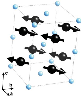
FIG. 5. (Color online) The G-type magnetic structure of \( EuTiO_{3} \) as determined by neutron and x-ray magnetic diffraction. Big (black) spheres represent the Eu ions, small (light blue) spheres represent the Ti atoms. Oxygen atoms are not shown for clarity. The black arrows illustrate the direction of the Eu magnetic moments.
if we were to postulate that the moments were along the [100] direction (see the dotted line in Fig. 4), we cannot account for the observed experimental modulations having \( \chi^{2} > 1000 \) . Simulations with magnetic moments between the [100] and [110] resulted in \( \chi^{2} > 300 \) . We can then conclude that the magnetic moments lie along the [110] direction within \( \pm5 \) deg. Such results are in agreement with recent calculations for a three-dimensional Heisenberg model. \( ^{65} \) The proposed motif for the magnetic moments is illustrated in Fig. 5.
Finally, we comment on recent experiments that have proposed the existence of another critical temperature \( T^{*} = 2.75 \, K \) . \( ^{65} \) It is suggested that above this temperature the magnetic moment easy axis flops from the a,b plane to the c axis. The existence of such a phase has been revealed by poling the sample under electric field, which effectively creates a monodomain sample. Figure 1 illustrates a difference pattern resulting from neutron diffraction between 2 and 3 K. Our neutron experiments below \( T^{*} \) cannot prove or disprove the flop of the magnetic moments, given that the powder diffractogram is consistent with both magnetic moment orientations. However, we do not observe any significant change of the structural reflections below the Néel temperature and close to \( T^{*} \) or any anomaly in the magnetic diffracted intensity. Therefore, our diffraction measurements suggest that in the unpoled sample the magnetic moments stay within the a,b plane, even above \( T^{*} \) . In this respect, results from Petrovic et al. \( ^{65} \) suggest an appealing possibility to manipulate the Eu spins through an applied external electric field.
IV. CONCLUSION
We have combined neutron powder diffraction and magnetic resonant x-ray diffraction to study the magnetic structure of \( EuTiO_{3} \) . We find that the magnetic moments order in an antiferro G-type motif, with the moments lying within the a,b
plane along the plane diagonal. The Eu magnetic moment value is compatible with the one expected for a free ion. Moreover, our neutron powder diffraction patterns suggest the absence of any further transition below the Néel temperature, for a sample not poled in electric field. Further experiments in applied electric field are planned to scrutinize the report of the low temperature spin-flop phase.
\( ^{*} \) valerio.scagnoli@psi.ch
\( ^{1} \) W. Eerenstein, N. D. Mathur, and J. F. Scott, Nature (London) 442, 759 (2006).
\( ^{2} \) T. Kimura, T. Goto, H. Shintani, K. Ishizaka, T. Arima, and Y. Tokura, Nature (London) 426, 55 (2003).
\( ^{3} \) T. Lottermoser, T. Lonkai, U. Amann, D. Hohlwein, J. Ihringer, and M. Fiebig, Nature (London) 430, 541 (2004).
\( ^{4} \) J. Wang, J. B. Neaton, H. Zheng, V. Nagarajan, S. B. Ogale, B. Liu, D. Viehland, V. Vaithyanathan, D. G. Schlom, U. V. Waghmare, N. A. Spaldin, K. M. Rabe, M. Wuttig, and R. Ramesh, Science 299, 1719 (2003).
\( ^{5} \) A. Zvezdin and A. Pyatakov, Usp. Fiz. Nauk 174, 465 (2004).
\( ^{6} \) A. Pimenov, A. A. Mukhin, V. Y. Ivanov, V. D. Travkin, A. M. Balbashov, and A. Loidl, Nat. Phys. 2, 97 (2006).
7 J. F. Scott, Nat. Mater. 6, 256 (2007).
\( ^{8} \) A. Zvezdin, A. Logginov, G. Meshkov, and A. Pyatakov, Bull. Rus. Acad. Sci. 71, 1561 (2007).
\( ^{9} \) K. Fujita, N. Wakasugi, S. Murai, Y. Zong, and K. Tanaka, Appl. Phys. Lett. 94, 062512 (2009).
\( ^{10} \) C. J. Fennie and K. M. Rabe, Phys. Rev. Lett. 97, 267602 (2006).
\( ^{11} \) J. H. Lee, L. Fang, E. Vlahos, X. Ke, Y. W. Jung, L. F. Kourkoutis, J.-W. Kim, P. J. Ryan, T. Heeg, M. Roeckerath, V. Goian, M. Bernhagen, R. Uecker, P. C. Hammel, K. M. Rabe, S. Kamba, J. Schubert, J. W. Freeland, D. A. Muller, C. J. Fennie, P. Schiffer, V. Gopalan, E. Johnston-Halperin, and D. G. Schlom, Nature (London) 466, 954 (2010).
\( ^{12} \) J. Brou, I. Fankuchen, and E. Banks, Acta Crystallogr. 6, 67 (1953).
\( ^{13} \) M. Allieta, M. Scavini, L. J. Spalek, V. Scagnoli, H. C. Walker, C. Panagopoulos, S. S. Saxena, T. Katsufuji, and C. Mazzoli, Phys. Rev. B 85, 184107 (2012).
\( ^{14} \) A. Bussmann-Holder, J. Köhler, K. R. Kremer, and J. M. Law, Phys. Rev. B 83, 212102 (2011).
\( ^{15} \) T. R. McGuire, M. W. Shafer, R. J. Joenk, H. A. Alperin, and S. J. Pickart, J. Appl. Phys. 37, 981 (1966).
\( ^{16} \) T. Katsufuji and H. Takagi, Phys. Rev. B 64, 054415 (2001).
\( ^{17} \) V. V. Shvartsman, P. Borisov, W. Kleemann, S. Kamba, and T. Katsufuji, Phys. Rev. B 81, 064426 (2010).
\( ^{18} \) K. A. Müller and H. Burkard, Phys. Rev. B 19, 3593 (1979).
\( ^{19} \) G. A. Gehring, Ferroelectrics 161, 275 (1994).
\( ^{20} \) A. D. Christianson, M. D. Lumsden, M. Angst, Z. Yamani, W. Tian, R. Jin, E. A. Payzant, S. E. Nagler, B. C. Sales, and D. Mandrus, Phys. Rev. Lett. 100, 107601 (2008).
\( ^{21} \) M. Angst, R. P. Hermann, A. D. Christianson, M. D. Lumsden, C. Lee, M.-H. Whangbo, J.-W. Kim, P. J. Ryan, S. E. Nagler, W. Tian, R. Jin, B. C. Sales, and D. Mandrus, Phys. Rev. Lett. 101, 227601 (2008).
\( ^{22} \) A. M. Mulders, S. M. Lawrence, U. Staub, M. Garcia-Fernandez, V. Scagnoli, C. Mazzoli, E. Pomjakushina, K. Conder, and Y. Wang, Phys. Rev. Lett. 103, 077602 (2009).
ACKNOWLEDGMENTS
We would like to thank E. Suard and T. Hansen for their advice and for the excellent support during the neutron diffraction experiments. We also acknowledge insightful contributions from J. Blanco and V. Yu. Pomjakushin. This work has been supported by the Swiss National Science Foundation, NCCR MaNEP.
\( ^{23} \) E. Schierle, V. Soltwisch, D. Schmitz, R. Feyerherm, A. Maljuk, F. Yokaichiya, D. N. Argyriou, and E. Weschke, Phys. Rev. Lett. 105, 167207 (2010).
\( ^{24} \) R. D. Johnson, L. C. Chapon, D. D. Khalyavin, P. Manuel, P. G. Radaelli, and C. Martin, Phys. Rev. Lett. 108, 067201 (2012).
\( ^{25} \) M. Matsubara, Y. Shimada, K. Ohgushi, T. Arima, and Y. Tokura, Phys. Rev. B 79, 180407 (2009).
\( ^{26} \) M. Kenzelmann, A. B. Harris, S. Jonas, C. Broholm, J. Schefer, S. B. Kim, C. L. Zhang, S.-W. Cheong, O. P. Vajk, and J. W. Lynn, Phys. Rev. Lett. 95, 087206 (2005).
\( ^{27} \) D. Mannix, D. F. McMorrow, R. A. Ewings, A. T. Boothroyd, D. Prabhakaran, Y. Joly, B. Janousova, C. Mazzoli, L. Paolasini, and S. B. Wilkins, Phys. Rev. B 76, 184420 (2007).
\( ^{28} \) J. Voigt, J. Persson, J. W. Kim, G. Bihlmayer, and T. Brückel, Phys. Rev. B 76, 104431 (2007).
\( ^{29} \) S. B. Wilkins, T. R. Forrest, T. A. W. Beale, S. R. Bland, H. C. Walker, D. Mannix, F. Yakhou, D. Prabhakaran, A. T. Boothroyd, J. P. Hill, P. D. Hatton, and D. F. McMorrow, Phys. Rev. Lett. 103, 207602 (2009).
\( ^{30} \) H. C. Walker, F. Fabrizi, L. Paolasini, F. de Bergevin, J. Herrero-Martin, A. T. Boothroyd, D. Prabhakaran, and D. F. McMorrow, Science 333, 1273 (2011).
\( ^{31} \) L. C. Chapon, P. G. Radaelli, G. R. Blake, S. Park, and S.-W. Cheong, Phys. Rev. Lett. 96, 097601 (2006).
\( ^{32} \) P. G. Radaelli, L. C. Chapon, A. Daoud-Aladine, C. Vecchini, P. J. Brown, T. Chatterji, S. Park, and S.-W. Cheong, Phys. Rev. Lett. 101, 067205 (2008).
\( ^{33} \) S. Partzsch, S. B. Wilkins, J. P. Hill, E. Schierle, E. Weschke, D. Souptel, B. Büchner, and J. Geck, Phys. Rev. Lett. 107, 057201 (2011).
\( ^{34} \) R. A. de Souza, U. Staub, V. Scagnoli, M. Garganourakis, Y. Bodenthin, S.-W. Huang, M. Garcia-Fernandez, S. Ji, S.-H. Lee, S. Park, and S.-W. Cheong, Phys. Rev. B 84, 104416 (2011).
\( ^{35} \) T. Katsufuji and Y. Tokura, Phys. Rev. B 60, R15021 (1999).
\( ^{36} \) J. Rodríguez-Carvajal, Phys. B: Cond. Matt. 192, 55 (1993).
\( ^{37} \) E. F. Bertaut, J. Phys. Colloq. 32, C1 (1971).
\( ^{38} \) J. Rodríguez-Carvajal, BASIREPS: A program for calculating non-normalized basis functions of the irreducible representations of the little group \( G_{k} \) for atom properties in a crystal, Laboratoire Leon Brillouin, CEA Saclay, Gif sur Yvette, France, 2004.
\( ^{39} \) L. Paolasini, C. Detlefs, C. Mazzoli, S. Wilkins, P. P. Deen, A. Bombardi, N. Kernavanois, F. de Bergevin, F. Yakhou, J. P. Valade, I. Breslavetz, A. Fondacaro, G. Pepellin, and P. Bernard, J. Synchr. Rad. 14, 301 (2007).
\( ^{40} \) ID20 has regrettably stopped operations as a magnetic scattering beamline since May 2011.
\( ^{41} \) C. Mazzoli, S. B. Wilkins, S. Di Matteo, B. Detlefs, C. Detlefs, V. Scagnoli, L. Paolasini, and P. Ghigna, Phys. Rev. B 76, 195118 (2007).
\( ^{42} \) F. Vaillant, Acta Crystallogr. Sect. A 33, 967 (1977).
\( ^{43} \) V. Scagnoli, C. Mazzoli, C. Detlefs, P. Bernard, A. Fondacaro, L. Paolasini, F. Fabrizi, and F. de Bergevin, J. Synchr. Rad. 16, 778 (2009).
\( ^{44} \) C. Giles, C. Malgrange, J. Goulon, F. de Bergevin, C. Vettier, E. Dartyge, A. Fontaine, C. Giorgetti, and S. Pizzini, J. Appl. Crystallogr. 27, 232 (1994).
\( ^{45} \) C. Giles, C. Vettier, F. de Bergevin, C. Malgrange, G. Grubel, and F. Grossi, Rev. Sci. Instrum. 66, 1518 (1995).
\( ^{46} \) J. P. Hannon, G. T. Trammell, M. Blume, and D. Gibbs, Phys. Rev. Lett. 61, 1245 (1988).
\( ^{47} \) J. P. Hannon, G. T. Trammell, M. BLume, and D. Gibbs, Phys. Rev. Lett. 62, 2644 (1989).
\( ^{48} \) J. P. Hill and D. F. McMorrow, Acta Crystallogr. Sect. A 52, 236 (1996).
\( ^{49} \) D. Templeton and L. Templeton, Acta Crystallogr. Sect. A 38, 62 (1982).
\( ^{50} \) V. Dmitrienko, Acta Crystallogr. Sect. A 39, 29 (1983).
\( ^{51} \) D. Templeton and L. Templeton, Acta Crystallogr. Sect. A 42, 478 (1986).
\( ^{52} \) V. Scagnoli, U. Staub, A. M. Mulders, M. Janousch, G. I. Meijer, G. Hammerl, J. M. Tonnerre, and N. Stojic, Phys. Rev. B 73, 100409(R) (2006).
\( ^{53} \) H. Jang, J.-S. Lee, K.-T. Ko, W.-S. Noh, T. Y. Koo, J.-Y. Kim, K.-B. Lee, J.-H. Park, C. L. Zhang, S. B. Kim, and S.-W. Cheong, Phys. Rev. Lett. 106, 047203 (2011).
\( ^{54} \) S. Agrestini, C. Mazzoli, A. Bombardi, and M. R. Lees, Phys. Rev. B 77, 140403 (2008).
\( ^{55} \) We drop the bold style for \( \epsilon \) ( \( \epsilon' \) ) to \( \epsilon \) ( \( \epsilon' \) ) for the sake of simplicity.
\( ^{56} \) M. W. Haverkort, N. Hollmann, I. P. Krug, and A. Tanaka, Phys. Rev. B 82, 094403 (2010).
\( ^{57} \) S. B. Wilkins, J. A. Paixão, R. Caciuffo, P. Javorsky, F. Wastin, J. Rebizant, C. Detlefs, N. Bernhoeft, P. Santini, and G. H. Lander, Phys. Rev. B 70, 214402 (2004).
\( ^{58} \) S. W. Lovesey, E. Balcar, K. S. Knight, and J. F. Rodriguez, Phys. Rep. 411, 233 (2005).
\( ^{59} \) V. Scagnoli and S. W. Lovesey, Phys. Rev. B 79, 035111 (2009).
\( ^{60} \) Note that the notation for the Stokes parameters used in these latter references is different from ours and our parameters \( P_{1} \) , \( P_{2} \) , and \( P_{3} \) correspond to \( P_{3} \) , \( P_{1} \) , and \( P_{2} \) , respectively, in Refs. 61 and 62.
\( ^{61} \) S. W. Lovesey and S. P. Collins, X-ray Scattering and Absorption by Magnetic Materials (Clarendon, Oxford, 1996).
\( ^{62} \) J. Fernández-Rodríguez, S. W. Lovesey, and J. A. Blanco, Phys. Rev. B 77, 094441 (2008).
\( ^{63} \) The agreement between the observed and calculated intensity is estimated via \( \chi^{2}=\sum_{i}\{[y_{i}-f(x_{i})]/\sigma_{i}\}^{2}/(n_{p}-n_{\mathrm{par}}) \) , where \( y_{i} \) are the experimental data, \( f(x_{i}) \) are the calculated values, \( \sigma_{i} \) represent the error bars, \( n_{p} \) is the number of point measured, and \( n_{par} \) is the number of free parameter in the fit.
\( ^{64} \) The azimuthal angle scan and the linear polarization scan were performed using different experimental setups and therefore the part of the sample which was probed was not necessarily the same.
\( ^{65} \) A. Petrović, Y. Kato, S. Sunku, T. Ito, P. Sengupta, L. Spalek, M. Shimuta, T. Katsufuji, C. Batista, S. Saxena, and C. Panagopoulos, arXiv:1204.0150.
 p3_0.jpg
 p3_1.jpg
 p4_0.jpg
 p4_1.jpg
 p5_0.jpg