| Transition Temperature | 420 K |
|---|---|
| Experiment Temperature | 200 K |
| Propagation Vector | k1 (0, 0, 0) |
| Parent Space Group | P63/mmc (#194) |
| Magnetic Space Group | Cm'cm' (#63.464) |
| Magnetic Point Group | m'm'm (8.4.27) |
| Lattice Parameters | 5.66500 5.66500 4.53100 90.00 90.00 120.00 |
|---|---|
| DOI | 10.1088/0953-8984/2/47/015 |
| Reference | P.J. Brown, V. Nunez, F. Tasset, J.B. Forsyth and P. Radhakrishna, Journal of Physics: Condensed Matter (1990) 2 9409-9422. |
| Label | Element | Mx | My | Mz | |M| |
|---|---|---|---|---|---|
| Mn1_1 | Mn | -1.73 | 1.73 | 0.0 | 3.00 |
| Mn1_2 | Mn | 3.46 | 1.73 | 0.0 | 3.00 |
Title
Determination of the magnetic structure of \( Mn_{3}Sn \) using generalized neutron polarization analysis
Authors
P J Brown†, V Nunez†, F Tasset†, J B Forsyth‡ and P Radhakrishna§ † Institut Max von Laue-Paul Langevin, BP 156X, 38042 Grenoble, France ‡ Rutherford Appleton Laboratory, Chilton, Oxon OX11 0QX, UK § Laboratoire Leon Brillouin CEN Saclay, 91191 Gif-sur-Yvette, France
Materials Studied
The primary material studied is \( Mn_{3}Sn \). Specifically, the single crystal sample used was of nominal composition \( Mn_{3-x}Sn \), and the introduction refers to structural parameters for \( Mn_{3.34}Sn \). The paper also mentions isostructural intermetallic compounds \( Mn_{3}Ge \) and \( Mn_{3}Ga \) in the context of previous studies.
Key Information
- Crystal structure / space group: \( DO_{19} \) structure, space group \( P6_{3}/mmc \).
- Magnetic ordering type and temperature:
- Antiferromagnetic structure based on a triangular arrangement of manganese magnetic moment directions lying in the basal plane.
- Weak ferromagnetism observed.
- Néel temperature (\( T_{N} \)): 420 K (for \( Mn_{3.7}Sn \), mentioned in literature review).
- Transition below 50 K to a magnetic structure with a significant ferromagnetically aligned moment parallel to [001].
- \( T_{1} \) (temperature where weak ferromagnetism reduces to near zero): 150–270 K (reported range).
- \( T_{2} \) (temperature where magnetization again increases): 100–50 K (reported range).
- Propagation vector(s):
- For \( Mn_{3.7}Sn \), a propagation vector parallel to [001] with a period of about 45 Å was observed below \( T_{1} \).
- For the sample studied in this paper, at 200 K, "the satellite reflections characteristic of the incommensurate phase were not found, so it was concluded that this phase did not occur in the sample".
- Magnetic moments:
- Manganese moment at 200 K: \( 3.00(1)\mu_{B} \).
- Previous reported values: \( 1.78(2)\mu_{B} \) at 293 K (Tomiyoshi 1982); 2.4(2) \( \mu_{B} \) (Zimmer and Kré 1973).
- Small ferromagnetic moment: 0.003 \( \mu_{B}/Mn \) in the basal plane (Zimmer and Kré 1973).
- Below 50 K, a significant ferromagnetic moment parallel to [001] is observed, reaching some 5.3 emu g\(^{-1}\) at 4.2 K.
- Lattice parameters: For \( Mn_{3.34}Sn \) at room temperature: a = 5.665 Å, c = 4.531 Å.
- Other critical measured values:
- Mn atomic site parameter x = 0.8388(2).
- The magnetic structure is unambiguously determined to be the 'inverse triangle' structure, requiring three trigonal domains.
- Depolarization of the purely nuclear 002 reflection at 5 K indicates the presence of ferromagnetic domains with the moment parallel to [001].
Synthesis Method
The crystal used in the experiments was "kindly given to us by S Tomiyoshi: it had been quenched from \( 900^{\circ} \) C and was in the form of a disk cut perpendicular to c approximately 3 mm thick and 5 mm diameter." The paper does not describe the initial growth or preparation of the ingot from which this crystal was obtained.
Abstract
The newly developed technique of generalized polarization analysis has been used to re-examine the triangular magnetic structure of \( Mn_{3}Sn \). The magnitude and direction of the polarization of neutrons scattered by some mixed magnetic and nuclear Bragg reflections at 200 K have been measured for a range of different incident polarization directions using a zero-field polarimeter. The results have been used to discriminate between different models which have been proposed for the magnetic structure. The analysis shows unambiguously that a structure allowing three trigonal domains is necessary to account for the scattered polarizations. Of the models suggested up to now only the 'inverse triangle' structure satisfies this criterion. The manganese moment was determined to be \( 3.00(1)\mu_{B} \) much larger than the value \( (1.78\mu_{B}) \) given by earlier measurements of the flipping ratios in an applied field. On cooling below 50 K the polarization analysis gave evidence for a transition to a magnetic structure with a significant ferromagnetically aligned moment parallel to [001].
Main Content Summary
The paper investigates the complex magnetic behavior of \( Mn_{3}Sn \), an intermetallic compound with a \( DO_{19} \) structure (space group \( P6_{3}/mmc \)). Previous studies had established a triangular antiferromagnetic spin arrangement in the basal plane and weak ferromagnetism, but ambiguities remained regarding the precise spin orientation (e.g., parallel to [100] or [110]) and the role of magnetic domains. Conflicting values for the manganese magnetic moment (ranging from 1.78 \( \mu_B \) to 2.4 \( \mu_B \)) were also reported. The authors note that stoichiometry and thermal treatment significantly influence the magnetic properties, including the Néel temperature (\( T_N \)), the temperature at which weak ferromagnetism diminishes (\( T_1 \)), and the temperature at which magnetization increases again (\( T_2 \)).
To resolve these ambiguities, the authors employed the newly developed technique of generalized neutron polarization analysis using the CRYOPAD polarimeter. A key advantage of this method is that measurements are performed in zero external magnetic field, preventing external fields from influencing the domain structure. The technique involves measuring the magnitude and direction of scattered neutron polarization for various incident polarization directions, providing detailed information about the magnetic scattering tensor. The experimental procedure for determining the scattered polarization components was meticulously programmed and automated.
Measurements were first conducted at 200 K on a single crystal of \( Mn_{3-x}Sn \), a temperature at which the incommensurate phase was not observed in the sample. Analysis of polarization scans for reflections such as 100, 101, and 102 indicated that the magnetic structure factors are real and that the manganese moments lie within the basal plane. A qualitative assessment of the 100 reflection suggested that the magnetic interaction vector Q is oriented along the vertical [010] direction, and significant depolarization in the horizontal plane pointed to the presence of domains with oppositely directed Q vectors.
Further measurements were performed at lower temperatures, revealing a significant additional depolarization below approximately 50 K. This observation is consistent with an abrupt increase in the ferromagnetic moment. At 5 K, the 101 and 100 reflections showed almost complete depolarization. Crucially, even the purely nuclear 002 reflection exhibited depolarization of its components in the (001) plane, while components parallel to [001] were preserved. This finding strongly suggests the existence of ferromagnetic domains with a moment aligned parallel to [001], which aligns with previous magnetization data showing an increase in spontaneous magnetization along [001] below 100 K.
A quantitative analysis, utilizing tensor equations to relate incident and scattered polarizations and considering various magnetic structure models and domain populations, was performed. The results unambiguously demonstrated that a structure allowing three trigonal domains is essential to explain the observed scattered polarizations. Among the previously proposed models, only the 'inverse triangle' structure (models (c) and (f) in the paper) met this criterion. The refined manganese moment was determined to be \( 3.00(1)\mu_{B} \), a value significantly higher than earlier experimental results (e.g., 1.78 \( \mu_B \)) but in excellent agreement with recent theoretical predictions of approximately 3 \( \mu_B \). The study highlights the high accuracy of generalized polarization analysis in determining magnetic-to-nuclear scattering ratios, independent of domain populations.
Conclusion
There is essentially no difference in the goodness of fit between the observed and calculated polarizations for models (c) and (f). The reason for this is that, although there is significant imbalance in the populations of equivalent \( 180^{\circ} \) domains, the division of the crystal amongst the three trigonal domains is very nearly equal. It can be shown that in the case of exact equality no difference in the scattered polarizations would be predicted. The magnetic moment obtained in both cases is \( 3.00(1)\mu_{\mathrm{B}} \), very much larger than the value \( 1.78 \mu_{B} \) obtained by Tomiyoshi (1982) from his polarized neutron measurements on a magnetized sample.
A recent calculation by Sticht et al (1989) based on a local approximation to spin-density functional theory suggests that the magnetic moment on Mn should be \( \simeq3\mu_{B} \), in agreement with the value we find.
The final \( \chi^{2} \) is quite satisfactory, but suggests that some instrumental aberrations still remain so that the precision of the scattered polarization directions is overestimated. However, even at this level of development it is clear that the technique of generalized polarization analysis is capable of measuring the ratio of magnetic to nuclear scattering with an accuracy of around 0.5%. This level of accuracy is as good, if not better than that obtainable with the classical polarized neutron method, in cases where the ratio of magnetic to nuclear scattering is large. The technique has the added advantage that the amplitude of magnetic scattering is determined essentially independently of the domain populations.
The present experiment indicates unequivocally that the magnetic structure of \( Mn_{3}Sn \) is one allowing at least three domains and the results are completely compatible with the inverse triangle structure. The question of the easy magnetization direction in zero field and hence of the true magnetic space group remains unresolved, but it is possible that a unique answer could be obtained by using the present technique on a previously magnetized sample for which the trigonal domains should be unequally populated.
Determination of the magnetic structure of \( Mn_{3}Sn \) using generalized neutron polarization analysis
This article has been downloaded from IOPscience. Please scroll down to see the full text article.
1990 J. Phys.: Condens. Matter 2 9409
(http://iopscience.iop.org/0953-8984/2/47/015)
View the table of contents for this issue, or go to the journal homepage for more
Download details:
IP Address: 200.144.93.190
The article was downloaded on 20/07/2013 at 17:10
Please note that terms and conditions apply.
Determination of the magnetic structure of \( Mn_{3}Sn \) using generalized neutron polarization analysis
P J Brown†, V Nunez†, F Tasset†, J B Forsyth‡ and P Radhakrishna§
† Institut Max von Laue-Paul Langevin, BP 156X, 38042 Grenoble, France
‡ Rutherford Appleton Laboratory, Chilton, Oxon OX11 0QX, UK
§ Laboratoire Leon Brillouin CEN Saclay, 91191 Gif-sur-Yvette, France
Received 8 May 1990, in final form 6 August 1990
Abstract. The newly developed technique of generalized polarization analysis has been used to re-examine the triangular magnetic structure of \( Mn_{3}Sn \) . The magnitude and direction of the polarization of neutrons scattered by some mixed magnetic and nuclear Bragg reflections at 200 K have been measured for a range of different incident polarization directions using a zero-field polarimeter. The results have been used to discriminate between different models which have been proposed for the magnetic structure. The analysis shows unambiguously that a structure allowing three trigonal domains is necessary to account for the scattered polarizations. Of the models suggested up to now only the 'inverse triangle' structure satisfies this criterion. The manganese moment was determined to be \( 3.00(1)\mu_{B} \) much larger than the value \( (1.78\mu_{B}) \) given by earlier measurements of the flipping ratios in an applied field. On cooling below 50 K the polarization analysis gave evidence for a transition to a magnetic structure with a significant ferromagnetically aligned moment parallel to [001].
1. Introduction
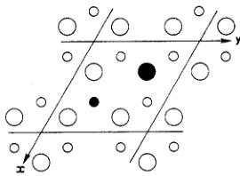
The complex magnetic behaviour of the isostructural intermetallic compounds with nominal compositions \( Mn_{3}Sn \) , \( Mn_{3}Ge \) and \( Mn_{3}Ga \) has been the subject of a number of studies since the first two of these compounds were shown to exhibit weak ferromagnetism by, respectively, Yasukochi et al (1961) and Ohoyama (1961). The basal plane projection of their \( DO_{19} \) structure, space group \( P6_{3}/mmc \) , is shown in figure 1. The atomic sites are:
| Atom | site | site symmetry | coordinates | ||
| Mn | 6h | mm | x | 2x | 1/4 |
| Metalloid | 2c | 6m2 | 1/3 | 2/3 | 1/4 |
The structure is generally stable only in the presence of excess Mn: in the Mn–Sn system, Mn atoms replace Sn to stabilize the structure over the range of composition \( Mn_{3.2}Sn-Mn_{3.7}Sn \) . For \( Mn_{3.34}Sn \) at room temperature the cell dimensions are a = 5.665, c = 4.531 Å and the value of the parameter x above is 0.8388(2) (Tomiyoshi 1982).
The first neutron diffraction measurements were made on polycrystalline samples of \( Mn_{3}Sn \) and \( Mn_{3}Ge \) by Kouvel and Kasper (1965) who deduced that their antiferromagnetic structures were based on a triangular arrangement of manganese magnetic moment directions lying in a plane containing [001]. They confirmed that the onset

Figure 1. The [001] projection of the \( DO_{1y} \) structure adopted by \( Mn_{3}Sn \) , \( Mn_{3}Ge \) and \( Mn_{3}Ga \) . Manganese atoms are shown as open circles, the larger being at height 1/4, the smaller at 3/4. The metalloid positions are shown as solid circles, the larger again being at height 1/4 and the smaller at 3/4.
of weak ferromagnetism in \( Mn_{3.7}Sn \) at 420 K coincided with the Néel temperature, \( T_{N} \) , and noted that its disappearance at around 220 K was accompanied by a splitting of the (101) magnetic reflection into a pair of satellites associated with a propagation vector parallel to [001] and a period of about 45 Å. This modulation persisted unchanged to 4.2 K but below 50 K they observed an upturn in the magnetization to a value greater than that observed in the temperature interval 270–420 K. Neutron powder diffraction experiments were also performed by Kré and Kádár (1970) on \( Mn_{3}Ga \) , by Kádár and Kré (1971) on \( Mn_{3}Ge \) and by Zimmer and Kré (1973) on \( Mn_{3}Sn \) . The latter authors confirmed the triangular nature of the spin arrangement at room temperature for a sample with 72.0(2) at% Mn ( \( Mn_{3.34}Sn \) ), but concluded that the moments of 2.4(2) \( \mu_{B} \) lay in the basal plane, as did the small ferromagnetic moment of 0.003 \( \mu_{B}/Mn \) . These authors also prepared single crystal samples of the same composition and found that annealing at temperatures between 550 and 800 °C was necessary to produce the long period modification of the magnetic structure first observed by Kouvel and Kasper (1965). Single crystal samples of \( Mn_{3.34}Sn \) were also prepared by Tomiyoshi (1982) who determined the polarization dependence of the scattered neutron intensity in \( \{h0l\} \) and \( \{hhl\} \) reflections with the sample at room temperature and in an 0.8 T field along [010] and [1–10] respectively. These data enabled him to confirm that the spin structure was indeed triangular with the spins in the basal plane but did not allow him to determine whether the spins lie parallel to [100] or [110]. The manganese moment was found to be 1.78(2) \( \mu_{B} \) at 293 K which extrapolates to some 2.1 \( \mu_{B} \) at 0 K. In a subsequent series of measurements Tomiyoshi and Yamaguchi (1982) claimed to have resolved the structural ambiguity through measurement of the flipping ratios as a function of rotations of the specimen about the scattering vector, again in an external field of 0.8 T. They concluded that the structure corresponds to the 'inverse triangle' model first proposed by Zimmer and Kré (1973).
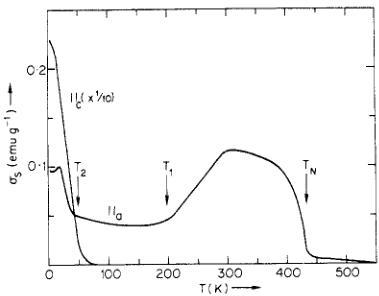
As a result of the measurements already referred to and additional single crystal studies by Ohmori et al (1987) and Tomiyoshi et al (1986 and 1987), it is clear that both stoichiometry and thermal treatment influence the magnitude of the weak ferromagnetism which appears below \( T_{N} \) , the temperature \( T_{1} \) at which this weak ferromagnetism reduces to near zero, the appearance or not of the incommensurate magnetic phase below \( T_{1} \) , the temperature \( T_{2} \) at which the magnetization again begins to increase and its maximum low temperature value (see figure 2). \( T_{1} \) has been reported in the range 150–270 K and \( T_{2} \) in the range 100–50 K. The magnetization below \( T_{2} \) is greatest along [001] and amounts to some 5.3 emu g \( ^{-1} \) at 4.2 K; however, Tomiyoshi et al (1986) could detect no significant changes in the integrated neutron intensities for a number of low angle magnetic reflections in the temperature range 4.2–100 K.
The object of the present experiment was to see to what extent the use of generalized polarization analysis would enable us to determine the exact nature of the triangular

Figure 2. The temperature dependence of the spontaneous magnetization parallel ( \( \parallel \) ) and perpendicular ( \( \perp \) ) to the c axis of the sample of \( Mn_{3-x}Sn \) used in the present experiments (Ohmori 1986).
structure, its domains and the magnitude of the Mn moment. One advantage of the technique is that the specimen is in zero external magnetic field, so its domain structure remains constant throughout the experiment. This is in contrast to the polarized beam experiments of Tomiyoshi (1982) and Tomiyoshi and Yamaguchi (1982) in which the magnetizing field of 0.8 T was known to influence the domain structure, but to an extent which was difficult to determine and which could influence the magnitude of the moment contributing to the observed flipping ratios. We have also made measurements down to 5 K and, for the first time, observed gross effects in the neutron scattering associated with the phase stable below \( T_{2} \) .
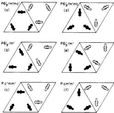
2. Models for the magnetic structures of \( DO_{10} \) compounds
The magnetic structures that are compatible with the symmetry of the \( DO_{19} \) structure and its sub-groups have been discussed by Zimmer and Krén (1973) and by Tomiyoshi (1982). Their results may be summarized as follows. The structures that retain the full symmetry \( 6_{3}/mmc \) are (1) the ferromagnetic one with all spins parallel to c, (2) a group of structures in which spins related by the inversion structure are oppositely directed, and (3) the two triangular structures of figure 3(a) and (d). All these structures may be rejected on the basis of experimental evidence, the first from the magnetization the second from the absence of a 111 reflection in the diffraction pattern, and the third from the presence of both 100 and 110 reflections in the patterns. Structures which are compatible with the powder diffraction intensities can be obtained by relaxing the symmetry in either of two ways. One possibility is to remove the mirror symmetry perpendicular to \( \langle100\rangle \) in the magnetic structures. This allows the spins to have a general orientation in the \( (001) \) planes so that both 100 and 110 reflections can occur; their relative intensities depend on the absolute spin orientation. The relative orientations of the spins for two particular cases in which the spins are in \( \langle100\rangle \) and \( \langle1-10\rangle \) directions are illustrated in figure 3(b) and 3(e) respectively. Alternatively the hexagonal symmetry axis may be reduced to just a diad. This gives the two structures 3(c) and 3(f), both of which have orthorhombic magnetic symmetry. Other structures with yet lower symmetry are possible. However, both the structures with reduced hexagonal \( (6/m) \) symmetry and the orthorhombic 'inverse triangle' structures are able to account for the observed magnetic diffraction, and indeed predict very similar diffraction intensities. Finally only the structures with orthorhombic symmetry, which allow inequivalence between the manganese atoms, are compatible with the weak ferromagnetism which is observed in the \( (001) \) plane.

Figure 3. Some of the possible spin configurations allowed by the full symmetry of the \( DO_{1/3} \) structure \( (P6_{3}/mmc) \) and its subgroups. In (a), (b) and (c) the spins are parallel to \( \langle100\rangle \) whereas in (d), (e) and (f) they are parallel to \( \langle110\rangle \) . The heavily shaded arrows show the spin directions on the Mn atoms at height 1/4, and the lightly shaded ones those on atoms at height 3/4.
Domains will be present in magnetic structures which have symmetry lower than that of the paramagnetic phase and the number of different domains will be equal to the order of the symmetry element which is relaxed. More generally, if the symmetry of the paramagnetic group is G and that of the magnetic group M, then there exists a subgroup S such that \( S \times M = G \) and the number of different domains is given by the order of S. In calculating magnetic diffraction intensities the average over all domains must be taken, and it is due to this averaging that both 100 and 110 reflections are predicted for the (c) and (f) structures above. It is particularly important to take proper account of the different domains when discussing the polarization analysis results.
3. The technique of generalized polarization analysis
Our measurements have been made using the CRYOPAD polarimeter described by Tasset et al (1988) and by Tasset (1989). The heart of the device is a liquid helium cryostat fitted with a variable temperature insert in which the specimen temperature may be set in the range 2–300 K. The specimen can be rotated about the vertical axis under the control of a dedicated PDP11/73 computer. The specimen chamber is surrounded by two concentric superconducting Meissner screens between which are two superconducting solenoids with their axes vertical, one fixed to intercept the incident neutron beam and the other, moveable, to intercept the Bragg scattered beam. The screens are cooled below their superconducting transition temperature in a shielded region of zero magnetic field. Outside this cryostat, the incident and scattered neutron beams pass through adiabatic spin-field rotators. On the incident side, the polarized beam from the parent IN20 triple axis spectrometer at the Institut Laue–Langevin, Grenoble first passes down a tubular collimator containing a longitudinal magnetic guide field and then enters a region of transverse field. The angle between this field and the vertical can be set by the computer to any desired nutation angle \( \theta \) . In the scattered beam the sequence of fields is reversed—first transverse, then longitudinal—before the beam enters the graphite
filter, Mezei spin flipper, Heusler alloy analyser and detector which are all part of the normal IN20 configuration.
The incident beam polarization at the sample position can be set to any desired direction by a suitable combination of nutation angle \( \theta \) and current in the vertical coil which causes the polarization to precess by an angle \( \Phi \) while passing between the outer and inner Meissner shields. Similarly, only appropriate choices of \( \Phi \) and \( \theta \) in the scattered beam will deliver the full scattered polarization parallel to the horizontal magnetization direction of the analyser. In addition to calculating the setting the rotation angle for the specimen, the CRYOPAD computer can position the output precession coil, set the required values of input and output \( \theta \) and \( \Phi \) , instruct IN20 to set the appropriate angles for analyser and detector and then carry out a flexible sequence of measurements at the desired specimen temperature.
A special technique has been developed to determine the scattered polarization corresponding to a given incident polarization (or vice-versa) which proceeds as follows. First the ratio R between the counting rates for flipper on and off is measured for three settings of the output angles: \( \Theta_{out} = 90^{\circ} \phi_{out} = 0 \) , \( \Theta_{out} = 90^{\circ} \phi_{out} = -90^{\circ} \) , \( \Theta_{out} = 0^{\circ} \phi_{out} = 0^{\circ} \) . The corresponding polarizations given by \( (1 - R)/(1 + R) \) give the components of the scattered polarization \( P_{X} \) , \( P_{Y} \) , \( P_{Z} \) where Y is parallel to the diffracted beam, Z is vertical and X completes a right-handed orthogonal set. These three measurements are used to estimate the precession \( \phi_{out} = \phi_{m} = 180 - \tan^{-1}(P_{Y}/P_{X}) \) after which, with \( \Theta_{out} = 90^{\circ} \) , the polarization would be positive and maximized. With \( \Theta_{out} = 90^{\circ} \) , R is again measured for a few values of \( \phi_{out} \) near to \( \phi_{m} - 90^{\circ} \) . At this position the polarization should be nearly zero and the dependence of P on \( \phi_{out} \) linear with a slope of \( \sqrt{(P_{X}^{2} + P_{Y}^{2})} \) radians \( ^{-1} \) . These data may therefore be used to find the precession \( \phi_{out} = \phi_{0} \) at which P = 0 with good precision. With \( \phi_{out} = \phi_{0} + 90^{\circ} \) a similar procedure is used to locate the position \( \Theta_{out} = \Theta_{0} \) at which the polarization is again zero using \( \Theta_{0} \cos^{-1}(P_{Z}/\sqrt{(P_{X}^{2} + P_{Y}^{2} + P_{Z}^{2})}) - 90^{\circ} \) and knowing that the gradient of P with respect to \( \Theta_{out} \) at this point is \( \sqrt{(P_{X}^{2} + P_{Y}^{2} + P_{Z})} \) radians \( ^{-1} \) . Finally with \( \Theta_{out} = \Theta_{0} + 90^{\circ} \) and \( \phi_{out} = \phi_{0} + 90^{\circ} \) measurement of R gives the magnitude of the scattered polarization which has spherical polar coordinates \( \Theta = \Theta_{0} + 90^{\circ} \) , \( \phi = 90^{\circ} - \phi_{0} \) with respect to the X, Y, Z axes defined above. It can be shown that with this technique, and assuming instrumental aberrations are negligible, the uncertainty in any one component of the polarization is just the statistical uncertainty in the determination of the polarizations at the zero polarization points. This whole procedure has been programmed for the PDP11 computer, so that given a setting of either the input or output coils, the corresponding scattered or incident polarization can be measured automatically.
4. Experimental measurements
The crystal used in the present experiments was kindly given to us by S Tomiyoshi: it had been quenched from \( 900^{\circ} \) C and was in the form of a disk cut perpendicular to c approximately 3 mm thick and 5 mm diameter. The susceptibility and spontaneous magnetization of a sample from the same ingot have been measured by Ohmori (1986) and are shown in figure 2. The crystal was mounted with an \( \langle010\rangle \) axis vertical on the central axis of the CRYOPAD cryostat. At a temperature of 200 K the satellite reflections characteristic of the incommensurate phase were not found, so it was concluded that this phase did not occur in the sample and a series of measurements was made at 200 K. The crystal was set to the peaks of the reflections 100, \( 10\overline{1} \) , 10-1 and


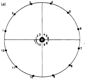
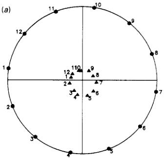
Figure 4. Stereographic projection of the incident and scattered polarization directions for the 100 (a) and 101 (b) reflections from Mn,Sn at 200 K. In (a) the incident polarization direction is being scanned in the (010) plane whilst in (b) it is scanned in the vertical plane containing the 101 scattering vector. The incident directions are marked by hexagons and the scattered directions by triangles, the filled symbols mark poles in the upper and open symbols those in the lower hemisphere. The number to the left of each symbol is the sequence number of the point in the scan and can be used to identify corresponding incident and scattered directions.
102 in turn. For each Bragg peak the direction of the input polarization was scanned, first in the plane perpendicular to the scattering vector \( (x) \) , then in the vertical plane containing x (y-scan) and finally in the horizontal plane (z-scan). Each scan was over a full \( 360^{\circ} \) in 13 steps of \( 30^{\circ} \) so that the first and last points were identical and gave a check on stability. At each point of the scan the magnitude and direction of the polarization of the diffracted beam were determined using the procedure explained above. The results of these measurements may be displayed by representing the input and output polarizations as points on a stereographic projection. Figure 4(a) shows the results of the z-scan of the 100 and 4(b) the y-scan of the \( 10\overline{1} \) reflection in this way. Such figures give a good qualitative appreciation of the rotation of the polarization of the scattered beam with respect to the incident beam, but to obtain quantitative information about the structure it is necessary to consider both the magnitude and direction of the polarization. In this context it is useful to define orthogonal axes x, y, z with x parallel to the scattering vector, z vertical (perpendicular to the incident and diffracted beams) and y completing the right-hand set; these are the axes of the polarization scans described above. The components, with respect to these axes, of both incident and scattered polarizations for selected points of the scans are tabulated in table 1 as a more quantitative record of the results obtained at 200 K.
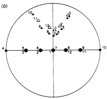
Another series of measurements was carried out at temperatures below 200 K. It was immediately found that a very significant additional depolarization took place on cooling below about 50 K. This is consistent with an abrupt increase in the ferromagnetic moment to a level at which depolarization in the domain walls becomes important. Figure 5 shows the temperature dependence of polarization scattered parallel to \( [010] \) by the 100 reflection for incident polarization also parallel to \( [010] \) ; it can be seen that between 60 K and 40 K a transition takes place in which all scattered polarization in this direction is lost.
Table I. Components of incident and diffracted polarization for the 100, 101 and 102 reflections of \( Mn_{3}Sn \) at 200 K. The axes are defined with x parallel to the scattering vector, z vertical and y completing the right-handed set.
| Incident polarization | Scattered polarization | ||||||||||
| Reflection 001 | Reflection 101 | Reflection 102 | |||||||||
| Px | Py | Pz | Px | Py | Pz | Px | Py | Pf | Pf | Pf | Pf |
| 0.00 | 0.00 | 0.88 | -0.02 | -0.01 | 0.78 | -0.02 | 0.32 | 0.49 | 0.04 | 0.38 | 0.54 |
| 0.44 | 0.00 | 0.76 | 0.00 | -0.01 | 0.67 | -0.10 | 0.28 | 0.44 | 0.15 | 0.38 | 0.43 |
| 0.76 | 0.00 | 0.44 | 0.02 | 0.00 | 0.42 | -0.13 | 0.33 | 0.25 | 0.21 | 0.37 | 0.24 |
| 0.88 | 0.00 | 0.00 | 0.03 | 0.00 | 0.09 | -0.14 | 0.34 | 0.06 | 0.22 | 0.38 | 0.03 |
| 0.76 | 0.00 | -0.44 | 0.33 | 0.01 | -0.25 | -0.13 | 0.37 | -0.13 | 0.19 | 0.39 | -0.18 |
| 0.44 | 0.00 | -0.76 | 0.04 | 0.01 | -0.06 | -0.07 | 0.40 | -0.31 | 0.11 | 0.44 | -0.40 |
| 0.00 | 0.88 | -0.01 | 0.01 | 0.03 | 0.13 | -0.01 | 0.33 | -0.07 | 0.01 | 0.57 | 0.06 |
| -0.01 | 0.76 | -0.45 | 0.00 | 0.04 | -0.22 | -0.01 | 0.35 | -0.07 | 0.01 | 0.57 | -0.09 |
| -0.01 | 0.43 | -0.77 | 0.02 | 0.03 | -0.57 | 0.00 | 0.37 | -0.23 | 0.00 | 0.56 | -0.27 |
| -0.02 | -0.01 | -0.88 | 0.02 | 0.01 | -0.75 | 0.01 | 0.41 | -0.38 | -0.02 | 0.47 | -0.45 |
| -0.01 | -0.45 | -0.76 | 0.01 | 0.00 | -0.60 | 0.02 | 0.42 | -0.39 | -0.04 | 0.27 | -0.50 |
| -0.01 | -0.77 | -0.43 | 0.00 | -0.03 | -0.26 | 0.03 | 0.39 | -0.17 | -0.05 | 0.02 | -0.24 |
| 0.00 | -0.88 | 0.01 | -0.01 | -0.04 | 0.10 | 0.04 | 0.35 | 0.14 | -0.04 | -0.09 | 0.18 |
| 0.01 | -0.76 | 0.45 | -0.01 | -0.04 | 0.42 | 0.01 | 0.34 | 0.42 | 0.01 | 0.02 | 0.52 |
| 0.01 | -0.43 | 0.77 | -0.02 | -0.02 | 0.67 | 0.00 | 0.33 | 0.53 | 0.03 | 0.21 | 0.63 |
| 0.02 | 0.01 | 0.88 | -0.01 | 0.01 | 0,78 | -0.01 | 0.33 | 0.49 | 0.03 | 0.39 | 0.54 |
| 0.01 | 0.45 | 0.76 | -0.04 | 0.00 | 0.69 | -0.01 | 0.32 | 0.36 | 0.02 | 0.49 | 0.37 |
| 0.01 | 0.77 | 0.43 | -0.01 | 0.03 | 0.45 | 0.00 | 0.32 | 0.21 | 0.02 | 0.54 | 0.21 |
To investigate the low temperature magnetic phase further, polarization scans of the 100, 101 and 002 reflections, similar to those made at 200 K, were carried out at 5 K. The results are summarized in table 2 which gives the components of incident and scattered polarization for a selection of points from the scans. The results for the 101 and 100 reflections are very similar and the scattered beam is almost completely

Figure 5. Polarization of the beam scattered by the 100 reflection as a function of temperature. The incident polarization is parallel to \( [010] \) .
depolarized. For the purely nuclear 002 reflection, however, the components of polarization in the \( (001) \) plane are destroyed whilst those parallel to \( [001] \) are preserved in all the scans. The components of polarization in table 2 are given on crystallographic axes to make this point clear. Such depolarization could arise from magnetic scattering by randomly populated antiferromagnetic domains if the magnetic scattering were much greater than the nuclear scattering; however, this cannot be the case for the 002 reflection which must have a zero magnetic structure factor for any antiferromagnetic arrangement of manganese spins. It seems more likely that the depolarization of the 002 reflection is due to the existence of ferromagnetic domains and their associated domain walls, with the ferromagnetic moment parallel to the direction in which the polarization is preserved namely \( [001] \) . If such is the case then the depolarization in the 101 and 100 reflections is due to the combination of that due to ferromagnetic and antiferromagnetic domains. Table 2 shows that what little polarization is scattered by these reflections is, as for the 002 reflection, parallel to \( [001] \) . The existence of a large ferromagnetic component of moment along \( [001] \) is in agreement with the observations of Ohmori et al (1987) and Tomiyoshi et al (1987) (figure 2) who find an increase in the spontaneous magnetization parallel to \( [001] \) below 100 K.
5. Determination of the structure from the scattered polarizations
The relationship between the incident and scattered polarizations \( P_{i} \) and \( P_{o} \) may be expressed by a tensor equation:
\[ \boldsymbol{P}_{o j}=\mathbf{A}_{i j}\boldsymbol{P}_{i j}+\boldsymbol{P}_{c i}. \quad (1) \]
In which the first term gives the rotation of the polarization which may be accompanied by a change of amplitude and the second term describes a polarization \( P_{c} \) which is created in the scattering process. The components of A and \( P_{c} \) can be calculated from the equation given by Blume (1963) as
\[ \mathbf{A}_{i j}=\left[\delta_{i j}(N N^{*}-\boldsymbol{Q}.\boldsymbol{Q}^{*})+2\mathrm{R e}(\boldsymbol{Q}_{i}\boldsymbol{Q}_{j}^{*})+2\mathrm{I m}(\epsilon_{i j k}(\boldsymbol{Q}_{k}N^{*}))\right]/I \quad (2) \]
\[ \boldsymbol{P}_{c i}=2\mathrm{R e}(\boldsymbol{Q}_{i}N^{*})+2\mathrm{I m}(\epsilon_{i j k}(\boldsymbol{Q}_{k}\boldsymbol{Q}_{j}^{*}))/I \quad (3) \]
\[ I=N N^{*}+2\mathrm{R e}(N\boldsymbol{P}.\boldsymbol{Q}^{*})+(\boldsymbol{Q}.\boldsymbol{Q}^{*})+\mathrm{i}[\boldsymbol{P}.(\boldsymbol{Q}\times\boldsymbol{Q}^{*})] \]
where N is the nuclear structure factor and Q the generalized magnetic interaction vector: \( \delta_{ij}=1 \) if i=j and is otherwise 0; \( \varepsilon_{ijk}=0 \) if any of the three indices are identical and is otherwise + or -1 depending on whether ijk is a cyclic permutation of xyz or not. I is a normalizing factor equal to the total scattered intensity.
It can be seen that only the third term in equation (2) can cause rotation of the polarization out of the Q-P plane and only the second term in equation (3) can create polarization perpendicular to Q. In none of the scans with input polarization in the plane perpendicular to the scattering vector was any significant component of the scattered polarization found to be out of this plane. This observation provides evidence that the magnetic structure factors are real in accordance with current models of the magnetic structure. A qualitative analysis of the scans of the 100 reflection indicates that Q for this reflection is along the vertical \( [010] \) direction and that a mixture of domains with oppositely directed Qs leads to the strong depolarization observed when the incident polarization is in the horizontal plane. This provides strong evidence that the moments have no component in the \( [001] \) direction: i.e. they lie in the basal plane in contradiction.
Table 2. Components of incident and scattered polarization for the 002, 101 and 100 reflections of \( Mn_{3}Sn \) at 5 K with respect to orthogonal crystallographic axes: (100), [010] and [001].
| Reflection | (002) | (101) | (100) | ||||||
| \( P_{a} \) | \( P_{b} \) | \( P_{c} \) | \( P_{a} \) | \( P_{b} \) | \( \mathbf{P}_{c} \) | \( P_{a} \) | \( P_{b} \) | \( P_{c} \) | |
| Input | 0.00 | 0.88 | 0.01 | 0.00 | 0.88 | 0.00 | 0.00 | 0.88 | 0.00 |
| Output | 0.05 | 0.14 | 0.05 | 0.04 | 0.06 | -0.10 | -0.02 | 0.01 | 0.00 |
| Input | 0.01 | 0.76 | 0.44 | 0.30 | 0.76 | 0.33 | 0.52 | 0.71 | 0.00 |
| Output | 0.05 | 0.09 | 0.45 | 0.01 | 0.05 | -0.16 | -0.02 | 0.01 | 0.00 |
| Input | 0.02 | -0.01 | 0.88 | 0.53 | 0.44 | 0.56 | 0.84 | -0.27 | 0.00 |
| 0.02 | -0.05 | 0.73 | -0.02 | 0.02 | -0.19 | -0.02 | 0.01 | 0.00 | |
| Input | 0.01 | -0.76 | 0.44 | 0.60 | 0.00 | 0.65 | 0.52 | -0.71 | 0.00 |
| Output | -0.03 | -0.14 | 0.36 | -0.02 | 0.00 | -0.19 | -0.02 | 0.00 | 0.00 |
| Input | 0.01 | 0.88 | 0.02 | 0.52 | -0.44 | 0.56 | 0.01 | 0.28 | 0.83 |
| 0.05 | 0.15 | 0.03 | -0.01 | -0.02 | -0.17 | -0.02 | 0.00 | -0.05 | |
| Input | 0.45 | 0.76 | 0.00 | 0.30 | -0.76 | 0.32 | 0.01 | 0.72 | 0.51 |
| 0.12 | 0.09 | 0.03 | -0.01 | -0.05 | -0.13 | -0.02 | 0.01 | -0.03 | |
| Input | -0.88 | 0.01 | 0.02 | -0.60 | 0.01 | 0.65 | 0.02 | 0.88 | -0.01 |
| -0.15 | 0.04 | -0.03 | -0.02 | 0.00 | -0.08 | -0.02 | 0.01 | 0.00 | |
| Input | -0.43 | 0.77 | 0.03 | -0.10 | 0.01 | 0.87 | 0.01 | 0.70 | -0.53 |
| -0.05 | 0.13 | 0.03 | -0.04 | 0.00 | -0.14 | -0.02 | 0.01 | 0.04 | |
| Input | -0.87 | 0.01 | 0.16 | 0.43 | 0.00 | 0.77 | 0.14 | 0.01 | 0.87 |
| -0.14 | 0.02 | 0.12 | -0.03 | 0.00 | -0.18 | -0.02 | 0.01 | -0.05 | |
| Input | -0.67 | 0.01 | 0.57 | 0.80 | -0.01 | 0.37 | 0.62 | 0.01 | 0.62 |
| -0.11 | 0.00 | 0.45 | 0.00 | 0.00 | -0.18 | -0.03 | 0.00 | -0.04 | |
| Input | 0.16 | -0.01 | 0.87 | 0.86 | -0.01 | -0.17 | 0.87 | 0.00 | 0.14 |
| 0.05 | -0.05 | 0.72 | 0.02 | 0.01 | -0.15 | -0.02 | 0.00 | -0.01 | |
| Input | 0.83 | -0.01 | 0.30 | 0.60 | -0.01 | -0.65 | 0.78 | -0.01 | -0.40 |
| 0.14 | -0.05 | 0.23 | 0.05 | 0.01 | -0.09 | -0.02 | 0.00 | 0.02 | |
to the original work of Kouvel and Kasper (1968) but in accord with the more recent studies.
A more quantitative analysis requires further development of the equations given above for the particular case of the triangular structures of figure 1. Table 3 lists the magnetic interaction vectors Q for h0l-type reflections for the six structures of figure 3. They are given in terms of \( \gamma \) , defined to be one half of the ratio between the magnetic and nuclear structure factors. As in section 4, orthogonal right-handed axes are defined with x parallel to the scattering vector and z vertical, so Q has only y and z components. In each case the Qs for all possible domains are given. Structures (a) and (d) have the full symmetry of the chemical space group, so the only domains are of the \( 180^{\circ} \) type for which the direction of all the spins are reversed and the phase of Q relative to that of the nuclear structure factor changes by \( 180^{\circ} \) . Structures (b) and (e) are those lacking the symmetry planes perpendicular to the \( \langle100\rangle \) and \( \langle1-10\rangle \) axes, so two domains related
Table 3. Magnetic interaction vectors Q of H-type reflections for the different magnetic structure models illustrated in figure 1. They are given in units of one half of the ratio of the magnetic to nuclear structure factors. The constant b = cos( \( \pi \) a / \( \left|k\right| \) \( \pi \) ). The constant b = cos( \( \pi \) a / \( \left|k\right| \pi \) ).
| Domain | Qc | Qc | Qc | Qc | Qc | Qe | Qe | Qe |
| 1 | 0 | 2γ | γ | 0 | 2γ | 2γ | 0 | 2γb |
| 2 | 0 | -2γ | -γ/γV3 | γ | -γ/γV3 | γ | -γb | γV3 |
| 3 | 0 | -2γ | -γ/γV3 | -γ | -γ/γV3 | -2γ | -γb | -γV3 |
| 4 | 0 | -2γ | -γ/γV3 | -2γ | -γ/γV3 | -2γ | -γb | -γV3 |
| 5 | 0 | -2γ | -γ/γV3 | -1 | -γ/γV3 | -1 | ||
| 6 | 0 | -2γ | -γ/γV3 | -3 | -γ/γV3 | -3 | -γb | -γV3 |
by these symmetry planes are present together with their \( 180^{\circ} \) partners. Structures (c) and (f) have three domains related by the missing triad axis, again each with its \( 180^{\circ} \) partner. The domains have been numbered so as to emphasize the relationship between the Qs for the different structures. Thus Q for domain 1 of structures (c) and (f) is the same as that for structures (a) and (d) respectively and the Qs for the domains (2 and 3) of (b) and (e) are identical to those of domains 2 and 3 of structures (c) and (f). Similar relationships for the general reflections explain why the different structures cannot be distinguished from intensity measurements alone.
In order to get an initial idea of how the scattered polarization depends on both the structure model and the domain populations, it is useful to calculate the scattered components of polarization in the principal directions \( (x, y, z) \) for polarization incident in each of these three principal directions in turn. It is convenient to express the domain populations \( \alpha_{n} \) (where \( \alpha_{n} \) is the fraction of the volume of the crystal in which the magnetic structure is that of domain n) in terms of the linear combinations:
\[ \begin{aligned}&c_{1}=\alpha_{1}+\alpha_{4}\quad&c_{3}=\alpha_{2}+\alpha_{3}+\alpha_{5}+\alpha_{6}\quad&c_{5}=\alpha_{2}-\alpha_{3}-\alpha_{5}+\alpha_{6}\\&c_{2}=\alpha_{1}-\alpha_{4}\quad&c_{4}=\alpha_{2}+\alpha_{3}-\alpha_{5}-\alpha_{6}\quad&c_{6}=\alpha_{2}-\alpha_{3}+\alpha_{5}-\alpha_{6}.\\ \end{aligned} \]
Defining \( P_{ij} \) as the component of scattered polarization parallel to i for incident polarization parallel to j and noting that for some models some of the coefficients \( \alpha \) are constrained to be zero, the following relationships can be deduced for models (a), (b) and (c):
\[ \begin{aligned}&P_{xx}=1-\gamma^{2}[4c_{1}+(3b^{2}+1)c_{3}]/D_{x}\\&P_{zx}=\gamma(2c_{2}+\sqrt{3}c_{4})/D_{x}\\&P_{xy}=0\\&P_{zy}=[2\sqrt{3}\gamma^{2}bc_{6}+\gamma(2c_{2}+\sqrt{3}c_{4})]/D_{y}\\&P_{xz}=0\\&P_{zz}=[1+\gamma^{2}[4c_{1}-(3b^{2}-1)c_{3}]+\gamma(2c_{2}+\sqrt{3}c_{4})]/D_{z}\\&P_{yx}=2\sqrt{3}\gamma bc_{5}/D_{x}\\&D_{x}=1+\gamma^{2}[4c_{1}+(3b^{2}+1)c_{3}]\end{aligned} \]
where \( \gamma \) is one half of the ratio of the magnetic to nuclear structure factors. \( D_{j} \) is proportional to the total scattered intensity with input polarization parallel to j. The constant \( b = \cos(\tan^{-1}(ha^{*}/1c^{*})) \) .
Similarly, for models \( (d) \) , \( (e) \) and \( (f) \) :
\[ \begin{aligned}&P_{xx}=[1-\gamma^{2}\{4b^{2}c_{1}+(b^{2}+3)c_{3}\}]/D_{x}\\&P_{zx}=2\sqrt{3}\gamma c_{4}\\&P_{xy}=0\\&P_{zy}=[2\sqrt{3}\dot{\gamma}^{2}bc_{6}+2\sqrt{3}\gamma c_{4}]/D_{y}\\ \end{aligned} \]
Table 4. Values of the polarizations measured in the three principal directions for the 101 reflection at 200 K.
| \( P_{ij} \) \( j \) \( i \) | x | y | z |
| x | -0.21 | 0.01 | 0.00 |
| y | 0.43 | 0.43 | 0.42 |
| z | 0.07 | 0.09 | 0.63 |
Table 5. Values of \( \gamma_{1011} \) , the constants \( c_{i} \) and the domain populations \( \alpha_{i} \) deduced from the polarizations in the three principal directions given in table 4. The columns labelled \( \alpha_{i}(\mathrm{LSQ}) \) give the results of the least squares analysis using all the measured data. The results for the models with spins parallel to \( \langle100\rangle \) (model (c)) and \( \langle110\rangle \) (model (f)) are given respectively in the left- and right-hand parts of the table. The moment per manganese atom is \( \gamma_{1011} \times 4.18 \) in Bohr magnetons.
| Model (c) | Model (f) | |||||
| i | c_{i} | \( \alpha_{i} \) | \( \alpha_{i}(\text{LSQ}) \) | c_{i} | \( \alpha_{i} \) | \( \omega_{i}(\text{LSQ}) \) |
| 1 | 0.32 | 0.24 | 0.191(7) | 0.30 | 0.30 | 0.331(7) |
| 2 | 0.15 | 0.38 | 0.333(8) | 0.30 | 0.33 | 0.275(7) |
| 3 | 0.68 | 0.06 | 0.049(4) | 0.70 | 0.06 | 0.115(4) |
| 4 | 0.19 | 0.09 | 0.144(4) | 0.07 | 0.00 | 0.00 |
| 5 | 0.57 | 0.00 | 0.00 | 0.46 | 0.06 | 0.060(13) |
| 6 | 0.07 | 0.25 | 0.283(12) | 0.08 | 0.25 | 0.219(6) |
| \( \gamma \) | 0.70 | 0.718(2) | 0.78 | 0.719(2) | ||
\[ \begin{aligned}&P_{xz}=0\\&P_{zz}=[1-\gamma^{2}\{4b^{2}c_{1}+(b^{2}-3)c_{3}\}+2\sqrt{3}\gamma c_{4}]/D_{z}\\&P_{yx}=2\gamma b(2c_{2}+c_{5})/D_{x}\\&D_{x}=1+\gamma^{2}[4b^{2}c_{1}+(b^{2}+3)c_{3}]\\&P_{yy}=\{1+\gamma^{2}[4b^{2}c_{1}+(b^{2}-3)c_{3}]+2\gamma b(2c_{2}+c_{5})/D_{y}\\&D_{y}=1+\gamma^{2}[4b^{2}c_{1}+(b^{2}-b^{2}+3)c_{3}]+2\gamma b(2c_{2}+c_{5})\\&P_{yz}=[2\sqrt{3}b\gamma^{2}c_{6}+2\gamma b(2c_{2}+c_{5})]/D_{z}\\&D_{z}=1+\gamma^{2}[4b_{2}c_{1}+(b^{2}+3)c_{3}]+2\sqrt{3}\gamma c_{4}.\\ \end{aligned} \]
These equations can be used to estimate values for \( \gamma \) and the domain populations which can subsequently be used as starting values in a least squares refinement involving all the measured polarizations.
The initial estimate of parameters is based on the observation that the \( P_{xx} \) term has the form \( (1 - q)/(1 + q) \) which allows q and hence \( D_{x} \) to be determined. The estimation of \( \gamma \) and the constants c is then straightforward. For the h0l reflections the constants \( c_{2} \) and \( c_{4} \) always occur in the combination \( 2c_{2} + \sqrt{3}c_{4} \) for the (c) structure and hence cannot be determined independently: the same type of relationship exists between \( c_{2} \) and \( c_{5} \) for structure (f). The measurements of the 101 reflection in the principal directions are given


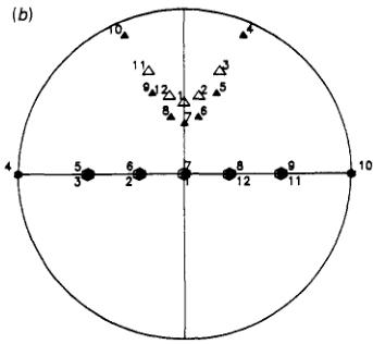
Figure 6. Stereographic projections of the directions of polarization scattered by the 100(a) and 101(b) reflections predicted from the refined structure model for incident polarization directions as in figure 4. The poles are marked in the same way as in figure 4.
in table 4 and values of the parameters for the two cases which have been estimated from them in table 5. Domain populations \( \alpha_{i} \) consistent with these values, subject to the constraints that \( 0 \leq \alpha \leq 1 \) for all the \( \alpha \) s and that the sum of all \( \alpha \) s must be unity are also shown in table 5. It should be noticed that for both sets of models the constants \( c_{1} \) and \( c_{3} \) are significantly different from zero indicating that only a three domain model, i.e. the 'inverse triangle' structures (c) and (f) will fit the data. The final columns of table 5 give the domain populations and the value of \( \gamma \) which have been refined from these values by making a least squares fit to the polarization scans of the 100, \( 10\overline{1} \) , 10-1 and 102 reflections. As pointed out, above the \( \alpha \) s are not all independently determined by the data so only four \( \alpha \) s are refined in each case: the fifth is given an arbitrary fixed value and the sixth determined by the normalization condition. The choice of which of the \( \alpha \) s to fix is nearly but not completely arbitrary: for instance setting \( c_{2} \) to zero ( \( \alpha_{1} = \alpha_{4} \) ) in model (f) leads to negative values for \( \alpha_{3} \) , \( \alpha_{5} \) and \( \alpha_{6} \) . In fact the high value of \( P_{yx} \) in table 4 suggests a large imbalance between domains 1 and 4 and therefore \( \alpha_{4} \) has been set to zero for model (f). Similar considerations suggest that the population of domain 5 for model (c) must be small and it has been fixed as zero. Fixing the smallest domain populations as zero avoids spurious values emerging from the least squares refinement.
The final values of \( \gamma \) and the domain parameters are listed in table 5 and the goodness of fit \( \chi^{2} \) calculated using the estimated values for the standard deviations of the components of polarization was 3.5 for both models (c) and (f). Figure 6 gives the stereographic projections of the incident and scattered polarization directions calculated from the model which are directly comparable with observed projections of figure 4.
6. Discussion
There is essentially no difference in the goodness of fit between the observed and calculated polarizations for models \( (c) \) and \( (f) \) . The reason for this is that, although there is significant imbalance in the populations of equivalent \( 180^{\circ} \) domains, the division of the crystal amongst the three trigonal domains is very nearly equal. It can be shown that in the case of exact equality no difference in the scattered polarizations would be predicted. The magnetic moment obtained in both cases is \( 3.00(1)\mu_{\mathrm{B}} \) , very much larger.
than the value \( 1.78 \mu_{B} \) obtained by Tomiyoshi (1982) from his polarized neutron measurements on a magnetized sample.
A recent calculation by Sticht et al (1989) based on a local approximation to spin-density functional theory suggests that the magnetic moment on Mn should be \( \simeq3\mu_{B} \) , in agreement with the value we find.
The final \( \chi^{2} \) is quite satisfactory, but suggests that some instrumental aberrations still remain so that the precision of the scattered polarization directions is overestimated. However, even at this level of development it is clear that the technique of generalized polarization analysis is capable of measuring the ratio of magnetic to nuclear scattering with an accuracy of around 0.5%. This level of accuracy is as good, if not better than that obtainable with the classical polarized neutron method, in cases where the ratio of magnetic to nuclear scattering is large. The technique has the added advantage that the amplitude of magnetic scattering is determined essentially independently of the domain populations.
The present experiment indicates unequivocally that the magnetic structure of \( Mn_{3}Sn \) is one allowing at least three domains and the results are completely compatible with the inverse triangle structure. The question of the easy magnetization direction in zero field and hence of the true magnetic space group remains unresolved, but it is possible that a unique answer could be obtained by using the present technique on a previously magnetized sample for which the trigonal domains should be unequally populated.
Acknowledgments
We would like to thank S Pujol for his help with the conception and construction of the CRYOPAD cryostat and J Alibon for the many modifications of the CRYOPAD software carried out on demand and at short notice.
References
Blume M 1963 Phys. Rev. 130 1670
Kádár G and Krén E 1971 Int. J. Magn. 1 143
Kouvel J S and Kasper J S 1965 Proc. Conf. on Magnetism (Nottingham, 1964) (London: Institute of Physics) p 169
Kréné E and Kádár G 1970 Solid State Commun. 8 1653
Nagamiya T, Tomiyoshi S and Yamaguchi Y 1982 Solid State Commun. 42 385
Ohmori H, Tomiyoshi S, Yamaguchi H and Yamamoto H 1987 J. Magn. Magn. Mater. 70 249
Ohmori H 1986 MSc Thesis Tohoku University (in Japanese)
Ohoyama T 1961 J. Phys. Soc. Japan 16 1995
Sticht J, Höck K-H and Kübler J 1989 J. Phys.: Condens. Matter 1 8155
Tasset F 1989 Physica B 156–157 627
Tasset F, Brown P J and Forsyth J B 1988 J. Appl. Phys. 63 3606
Tomiyoshi S 1982 J. Phys. Soc. Japan 51 803
Tomiyoshi S, Abe S, Yamaguchi Y, Yamaguchi H and Yamamoto H 1986 J. Magn. Magn. Mater. 54–57 1001
Tomiyoshi S and Yamaguchi Y 1982 J. Phys. Soc. Japan 51 2478
Tomiyoshi S, Yoshida H, Ohmori H, Kaneko T and Yamamoto H 1987 J. Magn. Magn. Mater. 70 247
Yasukochi K, Kanematsu K and Ohoyama T 1961 J. Phys. Soc. Japan 16 1123
Zimmer G J and Krén E 1972 Magnetism and Magnetic Materials 1971 (AIP Conf. Proc. No 5) (New York: American Institute of Physics) p 513
—— 1973 Magnetism and Magnetic Materials 1972 (AIP Conf. Proc. No 10) (New York: American Institute of Phys) p 1379
 p14_0.jpg
 p14_1.jpg
 p3_0.jpg
 p4_0.jpg
 p5_0.jpg
 p7_0.jpg
 p7_1.jpg
 p8_0.jpg