| Transition Temperature | 10.4 K |
|---|---|
| Parent Space Group | P4/mmm (#123) |
| Magnetic Space Group | Cm'cm' (#63.464) |
| Magnetic Point Group | m'm'm (8.4.27) |
| Lattice Parameters | 9.12960 9.12960 23.90600 90.00000 90.00000 90.00000 |
|---|---|
| DOI | 10.1103/physrevb.91.144404 |
| Reference | P. Äermak, K. Prokes, B. Ouladdiaf, M. Boehm, M. Kratochvilova and P. Javorsky, Physical Review B (2015) 91 144404. |
| Label | Element | Mx | My | Mz | |M| |
|---|---|---|---|---|---|
| Ho1_1 | Ho | 0.0 | 0.0 | 7.5 | 7.50 |
| Ho1_2 | Ho | 0.0 | 0.0 | -7.5 | 7.50 |
| Ho1_3 | Ho | 0.0 | 0.0 | 7.5 | 7.50 |
| Ho1_4 | Ho | 0.0 | 0.0 | 7.5 | 7.50 |
Title
Magnetic structures in the magnetic phase diagram of \( Ho_{2}RhIn_{8} \)
Authors
Petr Čermák, \( ^{1,2,*} \) Karel Prokeš, \( ^{3} \) Bachir Ouladdiaf, \( ^{4} \) Martin Boehm, \( ^{4} \) Marie Kratochvílová, \( ^{2} \) and Pavel Javorský \( ^{2} \)
\( ^{1} \) Jülich Centre for Neutron Science JCNS, Forschungszentrum Jülich GmbH, Outstation at MLZ, Lichtenbergstraße 1, 85747 Garching, Germany \( ^{2} \) Department of Condensed Matter Physics, Faculty of Mathematics and Physics, Charles University, Ke Karlovu 5, 121 16 Prague 2, The Czech Republic \( ^{3} \) Helmholtz-Zentrum Berlin für Materialien und Energie, Hahn-Meiner-Platz 1, Berlin 14109, Germany \( ^{4} \) Institut Laue Langevin, 6 rue Jules Horowitz, BP156, 38042 Grenoble Cedex 9, France
Materials Studied
\( Ho_{2}RhIn_{8} \)
Key Information
- Crystal structure / space group: Tetragonal, P4/mmm (No. 123).
- Magnetic ordering type and temperature:
- AF1: Antiferromagnetic ground state, orders below \( T_N = 10.9 \) K, transition to AF1 at \( T_1 = 10.4(2) \) K.
- AF2: Field-induced ferrimagnetic phase.
- AF3: Incommensurate zero-field phase, exists between \( T_N = 10.9 \) K and \( T_1 = 10.4 \) K.
- Propagation vector(s):
- AF1: \( \mathbf{k}=(1/2,0,0) \) (and \( \mathbf{k}'=(0,1/2,0) \) due to magnetic domains).
- AF2: \( \mathbf{k}_{0}=(0,0,0) \), \( \mathbf{k}_{1}=(1/2,0,0) \), \( \mathbf{k}_{2}=(0,1/2,1/2) \), \( \mathbf{k}_{3}=(1/2,1/2,1/2) \) (with corresponding domain vectors).
- AF3: Incommensurate with \( \mathbf{k}_{AF3}=(0.5,\delta,0) \), where \( \delta = 0.036(3) \).
- Magnetic moments:
- Ho magnetic moments point along the tetragonal c axis in every phase.
- AF1: \( \mu_{AF1} = 6.9(2)\mu_{B} \).
- AF2 (at 4 T): \( \mu_{\mathbf{k}_{0}} = 3.6(4)\mu_{B} \), \( \mu_{\mathbf{k}_{1}} = 3.7(3)\mu_{B} \), \( \mu_{\mathbf{k}_{2}} = -4.0(2)\mu_{B} \). Overall amplitude \( \mu_{AF2} = 7.5(5)\mu_{B} \).
- Lattice parameters: At T = 1.6 K: \( a = 4.5648(16) \) Å, \( c = 11.953(12) \) Å.
- Any other critical measured values:
- Extinction parameter: \( q = 9.4(1.8) \).
- Paramagnetic Curie temperature \( \theta_{p} \): -21.1(1) K (for [100]), -8.9(2) K (for [001]).
- Effective magnetic moment \( \mu_{\text{eff}} \): 10.08(2) \( \mu_{B} \) (for [100]), 10.57(2) \( \mu_{B} \) (for [001]).
- Molecular field coefficients \( \lambda \): -1.31 mol/emu (for [100]), -0.58 mol/emu (for [001]).
- Exchange interaction \( J_{\text{ex}} \): -0.68 K (for [100]), -0.78 K (for [001]).
- Crystal field parameters: \( B_{2}^{0} = -0.173 \) K, \( B_{4}^{0} = 1.08 \times 10^{-3} \) K, \( B_{4}^{4} = -1.27 \times 10^{-2} \) K, \( B_{6}^{0} = -3.35 \times 10^{-6} \) K, \( B_{6}^{4} = 9.70 \times 10^{-6} \) K.
Synthesis Method
The identical sample of \( Ho_{2}RhIn_{8} \) as in the previous bulk experiments [13] was used. The synthesis method itself is not described in this paper.
Abstract
The magnetic phase diagram of the tetragonal \( Ho_{2}RhIn_{8} \) compound has similar features to many related systems, revealing a zero magnetic field AF1 and a field-induced AF2 phases. Details of the magnetic order in the AF2 phase were not reported yet for any of the related compounds. In addition, only the \( Ho_{2}RhIn_{8} \) phase diagram contains a small region of the incommensurate zero-field AF3 phase. We have performed a number of neutron diffraction experiments on single crystals of \( Ho_{2}RhIn_{8} \) using several diffractometers including experiments in both horizontal and vertical magnetic fields up to 4 T. We present details of the magnetic structures in all magnetic phases of the rich phase diagram of \( Ho_{2}RhIn_{8} \) . The Ho magnetic moments point along the tetragonal c axis in every phase. The ground-state AF1 phase is characterized by propagation vector \( \mathbf{k}=(1/2,0,0) \) . The more complex ferrimagnetic AF2 phase is described by four propagation vectors \( \mathbf{k}_{0}=(0,0,0) \) , \( \mathbf{k}_{1}=(1/2,0,0) \) , \( \mathbf{k}_{2}=(0,1/2,1/2) \) , \( \mathbf{k}_{3}=(1/2,1/2,1/2) \) . The magnetic structure in the AF3 phase is incommensurate with \( \mathbf{k}_{AF3}=(0.5,\delta,0) \) . Our results are consistent with theoretical calculations based on crystal field theory.
Main Content Summary
This paper investigates the complex magnetic phase diagram of the tetragonal compound \( Ho_{2}RhIn_{8} \) using neutron diffraction experiments on single crystals. The study aims to elucidate the magnetic structures in its three distinct phases: the zero-field antiferromagnetic AF1 phase, the field-induced ferrimagnetic AF2 phase, and a unique incommensurate zero-field AF3 phase. While \( Ho_{2}RhIn_{8} \) shares similarities with other R-T-X compounds (R=rare earth, T=transition metal, X=In or Ga), the details of its AF2 phase were previously unknown, and the AF3 phase is a unique feature not observed in related "115" or "218" systems.
The experimental methodology involved comprehensive neutron diffraction measurements using various diffractometers (D10, CYCLOPS, E4, IN3) at ILL and HZB, covering both zero-field and applied magnetic fields up to 4 T, along with magnetic susceptibility measurements. The structural parameters were refined from D10 data, confirming the P4/mmm space group. Data analysis utilized programs like RACER, DATARED, and FULLPROF for integration, reduction, and refinement of magnetic structures.
The ground-state AF1 phase, observed below \( T_1 = 10.4(2) \) K, is characterized by a commensurate propagation vector \( \mathbf{k}=(1/2,0,0) \). The Ho magnetic moments are aligned along the tetragonal c-axis, with an amplitude of \( 6.9(2)\mu_{B} \). The presence of equally sized magnetic Bragg reflections for \( \mathbf{k}=(1/2,0,0) \) and \( \mathbf{k}'=(0,1/2,0) \) indicates the existence of two equally populated magnetic k-domains. This AF1 structure is noted to be more akin to "115" compounds than other "218" compounds, which typically exhibit a \( \mathbf{k}=(1/2,1/2,1/2) \) propagation.
The field-induced AF2 phase, established above 2.5 T, is a more complex ferrimagnetic structure described by multiple propagation vectors: \( \mathbf{k}_{0}=(0,0,0) \), \( \mathbf{k}_{1}=(1/2,0,0) \), \( \mathbf{k}_{2}=(0,1/2,1/2) \), and \( \mathbf{k}_{3}=(1/2,1/2,1/2) \). The Ho moments remain along the c-axis. The refinement yielded magnetic moment amplitudes of \( \mu_{\mathbf{k}_{0}} = 3.6(4)\mu_{B} \), \( \mu_{\mathbf{k}_{1}} = 3.7(3)\mu_{B} \), and \( \mu_{\mathbf{k}_{2}} = -4.0(2)\mu_{B} \), resulting in an overall amplitude of \( \mu_{AF2} = 7.5(5)\mu_{B} \) at 4 T. This structure is proposed to involve a spin-flip of 1/4 of the magnetic moments, representing the first detailed solution for an AF2 phase in this family of compounds.
A unique incommensurate AF3 phase was identified in a narrow temperature range between \( T_N = 10.9 \) K and \( T_1 = 10.4 \) K. This phase is characterized by the propagation vector \( \mathbf{k}_{AF3}=(1/2, \delta, 0) \) with \( \delta = 0.036(3) \), which is temperature-independent. The small incommensurate component suggests a spin-density-wave phase. Crystal field theory analysis of magnetic susceptibility data confirmed the strong magnetic anisotropy with the easy c-axis magnetization. The determined CEF parameters, particularly a smaller \( B_{2}^{0} \) value compared to related compounds, suggest competing easy axes, which could explain the unique anisotropic propagation in AF1 and the existence of the incommensurate AF3 phase.
Conclusion
We have determined the magnetic structures in \( Ho_{2}RhIn_{8} \) by means of neutron diffraction experiments. In the zero-field ordered state, the magnetic order is characterized by a single propagation vector \( \mathbf{k}_{AF1} = (1/2, 0, 0) \) with the antiferromagnetic coupling of Ho moments along the c axis and the amplitude of the magnetic moment \( 6.9(2)\mu_{B} \) . Before entering this ground-state commensurate phase, there exists a small temperature region where the incommensurate phase with propagation \( \mathbf{k}_{AF3} = (1/2, 0.036, 0) \) develops. Both existence of the additional incommensurate phase and the ground-state propagation vector anisotropic within ab plane are unique within the \( R_{n}T_{m}X_{3n+2m} \) series. Analysis of the temperature dependence of magnetic susceptibility revealed paramagnetic Curie temperatures and set of crystal field parameters, which are in agreement with observed anisotropic magnetic structures. These results confirm that magnetism in \( Ho_{2}RhIn_{8} \) is purely CEF driven. The mean-field theory model can be used for the estimation of the magnetic exchange constants and magnetic structures.
In the applied magnetic field along the c axis the magnetic structure transforms by spin flipping of the 1/4 of magnetic moments to another commensurate phase with the amplitude of magnetic moment \( 7.5(5)\mu_{B} \) (in B = 4 T). Similar flipping behavior is expected also in the other related compounds with the same phase diagram.
Magnetic structures in the magnetic phase diagram of \( Ho_{2}RhIn_{8} \)
Petr Čermák, \( ^{1,2,*} \) Karel Prokeš, \( ^{3} \) Bachir Ouladdiaf, \( ^{4} \) Martin Boehm, \( ^{4} \) Marie Kratochvílová, \( ^{2} \) and Pavel Javorský \( ^{2} \)
\( ^{1} \) Jülich Centre for Neutron Science JCNS, Forschungszentrum Jülich GmbH, Outstation at MLZ,
Lichtenbergstraße 1, 85747 Garching, Germany
\( ^{2} \) Department of Condensed Matter Physics, Faculty of Mathematics and Physics, Charles University,
Ke Karlovu 5, 121 16 Prague 2, The Czech Republic
\( ^{3} \) Helmholtz-Zentrum Berlin für Materialien und Energie, Hahn-Meiner-Platz 1, Berlin 14109, Germany
\( ^{4} \) Institut Laue Langevin, 6 rue Jules Horowitz, BP156, 38042 Grenoble Cedex 9, France
(Received 1 September 2014; revised manuscript received 11 March 2015; published 7 April 2015)
The magnetic phase diagram of the tetragonal \( Ho_{2}RhIn_{8} \) compound has similar features to many related systems, revealing a zero magnetic field AF1 and a field-induced AF2 phases. Details of the magnetic order in the AF2 phase were not reported yet for any of the related compounds. In addition, only the \( Ho_{2}RhIn_{8} \) phase diagram contains a small region of the incommensurate zero-field AF3 phase. We have performed a number of neutron diffraction experiments on single crystals of \( Ho_{2}RhIn_{8} \) using several diffractometers including experiments in both horizontal and vertical magnetic fields up to 4 T. We present details of the magnetic structures in all magnetic phases of the rich phase diagram of \( Ho_{2}RhIn_{8} \) . The Ho magnetic moments point along the tetragonal c axis in every phase. The ground-state AF1 phase is characterized by propagation vector \( \mathbf{k}=(1/2,0,0) \) . The more complex ferrimagnetic AF2 phase is described by four propagation vectors \( \mathbf{k}_{0}=(0,0,0) \) , \( \mathbf{k}_{1}=(1/2,0,0) \) , \( \mathbf{k}_{2}=(0,1/2,1/2) \) , \( \mathbf{k}_{3}=(1/2,1/2,1/2) \) . The magnetic structure in the AF3 phase is incommensurate with \( \mathbf{k}_{AF3}=(0.5,\delta,0) \) . Our results are consistent with theoretical calculations based on crystal field theory.
DOI: 10.1103/PhysRevB.91.144404
PACS number(s): 61.05.fm, 75.30.Kz, 64.70.Rh
I. INTRODUCTION
The heavy-fermion compounds have been attracting the scientific interest for almost two decades due to presence of magnetic order and unconventional superconductivity induced in the vicinity of the magnetic quantum critical point \( [1] \) . Both phenomena can coexist in broad ranges of the temperature-pressure-substitution phase diagrams \( [2] \) . Compounds with general composition \( R_{n}T_{m}X_{3n+2m} \) (where R = rare earth, T = transition metal, X = In or Ga, n and m are integers) provide, however, another possibility of tuning the system towards quantum criticality due to their layered structure. The structural dimensionality plays a crucial role in the character of a magnetic quantum critical point \( [3,4] \) . In general, the crystal structure consists of rare-earth (n) and transition metal (m) layers surrounded by cages of indium atoms. Different sequences of these layers along tetragonal c axis is reflected in various tetragonal structures with rich ground-state properties. In terms of anisotropy, the “218” structure (e.g., \( Ce_{2}RhIn_{8} \) [5] or \( Ce_{2}PdIn_{8} \) [6,7]) lies in between the well known quasi-2D “115” structure (e.g., \( CeCoIn_{5} \) [8], \( CeRhIn_{5} \) [9]) and the cubic \( CeIn_{3} \) structure. Recently, this dimensionality row was enriched by discovering “127” compounds ( \( CePt_{2}In_{7} \) [10]) and new structure types “3-1-11” and “5-2-19” [11,12], which represent an intermediate step between \( CeIn_{3} \) and the “218” compounds. As the superconductivity is observed only in cerium compounds, studies of non-Kondo materials have a crucial importance for understanding the magnetism in these systems.
\( Ho_{2}RhIn_{8} \) orders antiferromagnetically below \( T_{N} = 10.9 K \) and its magnetic properties are driven mainly by crystalline electric field (CEF) effects and the RKKY interaction [13]. When an external magnetic field is applied along the tetragonal c axis, \( Ho_{2}RhIn_{8} \) undergoes two successive magnetic phase transitions at 2 K. Above 2.5 T an intermediate magnetic phase is established and further increase of magnetic field up to 6 T results in the ferromagnetic order. It is interesting to note that the magnetization per formula unit in the AF2 phase is just a half of the moment found in the ferromagnetic phase as was shown by magnetization measurements [13]. The magnetic phase diagram of \( Ho_{2}RhIn_{8} \) (see Ref. [13] and Fig. 1) is qualitatively comparable to many other related “115” and “218” compounds with R = Nd, Tb, Dy, and Ho where the c axis is the easy magnetization axis: \( RRhIn_{5} \) [14], \( RCoIn_{5} \) [15], \( RCoGa_{5} \) [15], \( R_{2}RhIn_{8} \) [13,16], and \( R_{2}CoGa_{8} \) [17]. As well as for \( Ho_{2}RhIn_{8} \) , the magnetization per formula unit in the field-induced AF2 phase in all these compounds is half of the value in the ferromagnetic phase. The microscopic nature of the magnetic order in the AF1 phase was studied in \( RRhIn_{5} \) (R = Nd, Tb, Dy, Ho) [18], \( RCoGa_{5} \) (R = Tb, Ho) [19], \( R_{2}RhIn_{8} \) (R = Nd, Tb, Dy) [20], and \( R_{2}CoGa_{8} \) (R = Tb, Dy, Ho) [21,22], resulting in the commensurate propagation \( k_{115} = (1/2, 0, 1/2) \) in “115” compounds and \( k_{218} = (1/2, 1/2, 1/2) \) in “218” compounds. Magnetic structure in the AF2 phase was studied only by Hieu in his thesis [18] in \( NdRhIn_{5} \) and \( DyRhIn_{5} \) , however no conclusions from this measurements were given and magnetic structure in the AF2 phase remains unknown.
Despite sharing many similarities with the isostructural Nd, Tb, and Dy compounds, \( Ho_{2}RhIn_{8} \) shows a feature not observed in other related compounds: an additional magnetic phase existing in a narrow temperature region between \( T_{N} = 10.9 \) K and \( T_{1} = 10.4 \) K. The jump in specific heat at \( T_{1} \) is clearly pronounced and it was speculated, that this phase transition is connected with a formation of an incommensurate magnetic phase [13].
The present paper focuses on the determination of magnetic structures in all three magnetic phases of \( Ho_{2}RhIn_{8} \) using

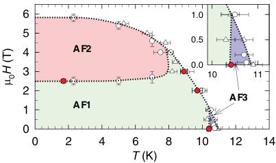
FIG. 1. (Color online) Magnetic phase diagram of \( Ho_{2}RhIn_{8} \) . Open points are determined from bulk measurements [13], filled ones are from current neutron diffraction studies. Lines and shapes are to guide the eye.
several neutron diffraction experiments. Considering the similar phase diagram and results of magnetization measurements, the magnetic structure in the AF2 phase might be then eventually generalized for the whole class of related “115” and “218” tetragonal compounds.
II. EXPERIMENTAL DETAILS
The identical sample of \( Ho_{2}RhIn_{8} \) as in the previous bulk experiments [13] was used. The single crystal has the form of a cuboid of approximately \( 3 \times 1 \times 0.2 \) mm size. No deviation from the known crystal structure (space group P4/mmm, No. 123) nor any presence of foreign phase were detected by x-ray diffractometer and EDX microprobe analysis. Magnetic susceptibility measurements were carried out with a physical property measurement system (PPMS-14) by Quantum Design with the Vibrating Sample Magnetometer option at Magnetism and Low Temperatures Laboratories in Prague.
Diffraction measurements were carried out on the several neutron diffractometers. First, the nuclear structure and the extinction parameters were determined by the D10 instrument at Institute Laue-Langevin (ILL). We used a PG002 monochromator with an incident wavelength \( \lambda = 2.36 \) Å and a graphite filter before the sample. The orientation matrix and lattice parameters were refined on the basis of 19 strong nuclear reflections at T = 2 K.
Determination of the propagation vectors in the AF1 and AF3 phases was done on Laue diffractometer CYCLOPS \( [23] \) at ILL. Measurement of two patterns with a different sample rotation at \( T = 14 K \) and in the ordered state at \( T = 1.6 K \) took three hours per pattern. In addition, a series of 50 patterns was taken in the slow temperature sweep mode (0.1 K/min) in order to determine temperature dependence of the magnetic Bragg peaks and the nature of the AF3 phase. Refinement of the Laue data were done in the Esmeralda Laue Suite program \( [24] \) .
The magnetic phase AF1, as well as the behavior in applied magnetic fields, were measured using the two-axis neutron diffractometer E4 at Helmholtz-Zentrum, Berlin, Germany. A focusing monochromator with vertically bent PG crystals was used for the wavelength \( \lambda = 2.432 \) Å. The scattered intensities were recorded using a \( 200 \times 200 \) mm two-dimensional position-sensitive detector (PSD) 896 mm from the sample. The experiment was performed using a He flow cryostat at the temperature range 1.6–15 K. First, the sample was loaded into a horizontal-field magnet, HM-2, and aligned with its reciprocal \( (h, 0, l) \) plane in the horizontal scattering plane of the instrument. The magnetic field was applied along the easy c axis. In order to extend the number of observable reflections, the sample was realigned and mounted to the vertical-field magnet, VM-2, to have \( (h, k, 0) \) plane aligned in the scattering plane of the instrument. The 10 degrees opening angle of the magnet allowed us to reach reflections with index \( (h, k, 0.5) \) on the PSD detector.
We used the triple axis spectrometer IN3 at ILL to measure zero-field temperature dependence of magnetic Bragg reflections. The sample was mounted similarly to the E4 experimental setup: with the reciprocal \( (h, 0, l) \) plane in the scattering plane and the experiment was performed in the elastic condition at \( \lambda = 2.36 \) Å.
III. RESULTS AND DISCUSSION
The data from D10 were integrated using the program RACER [25]. Integration of the E4 data was done by a PYTHON script; first cutting out background detector data to a rectangular shape around the observed reflection and then fitting a Gaussian profile along the \( \omega \) scan. This technique allows us to reduce the background and also to distinguish out-of-plane and in-plane reflections. Data from IN3 were fitted with a Gaussian profile, as this instrument has only a one-dimensional (1D) detector. All intensities were corrected for the Lorentz factor. The obtained raw data were reduced using the program DATARED [26] and the FULLPROF program [26] was used for the refinement of the structures.
The structural parameters of \( Ho_{2}RhIn_{8} \) were determined on the basis of 68 independent reflections measured on D10; they are summarized in Table I. A single extinction parameter q [27,28] was used in the FULLPROFsoftware for correction of extinction, resulting in \( q = 9.4(1.8) \) . This value combines both primary and secondary extinction proposed by Zachariasen [27] and is suitable for isotropic description of extinction effects. Extinction has not a negligible effect on strong magnetic reflections; the highest reduction of the intensity was observed for the reflection \( (1/2\ 0\ 1) \) , which was reduced by coefficient 0.69. As other neutron measurements were carried out using the same wavelength and the identical single crystal, this extinction parameter was used as a fixed value for all E4 and IN3 data refinements.
A. Zero-field commensurate structure AF1
All observed diffraction spots on the total Laue pattern obtained in the paramagnetic state can be indexed assuming
TABLE I. Refined structural parameters of \( Ho_{2}RhIn_{8} \) at \( T = 1.6 \) K. Space group: P4/mmm. \( a = 4.5648(16) \) Å, \( c = 11.953(12) \) Å.
| Atom | Wyckoff pos. | x | y | z |
| Ho | 2g | 0 | 0 | 0.3098(3) |
| Rh | 1a | 0 | 0 | 0 |
| In(1) | 2e | 0 | 0.5 | 0.5 |
| In(2) | 2h | 0.5 | 0.5 | 0.3086(6) |
| In(3) | 4i | 0 | 0.5 | 0.1245(4) |

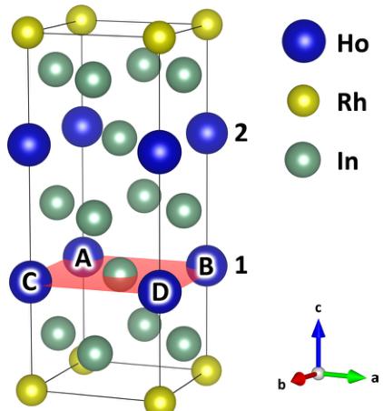
FIG. 2. (Color online) Crystal structure of the \( Ho_{2}RhIn_{8} \) compound.
a tetragonal structure with the space group P4/mmm. Their intensity remains unchanged when cooling to the ordered state at \( T = 1.5 \, K \) , showing no ferromagnetic or \( \mathbf{k} = (0,0,0) \) contribution to the magnetic structure in AF1. A large number of purely magnetic reflections appears in the ordered state; all of them can be described by a single propagation vector associated with the X \( [k = (1/2,0,0) \) and \( k' = (0,1/2,0)] \) point of symmetry. There exist eight one-dimensional (1D) irreducible representations associated with this wave vector, but only six of them are part of the global reducible magnetic representation of the 2g Wyckoff site occupied by Ho atoms. These can be assigned to six possible magnetic structures with the magnetic moments aligned along one of the main crystallographic directions, each with ferromagnetic or antiferromagnetic stacking of the moments on the two Ho positions within the unit cell (positions 1 and 2 in Fig. 2). All possible structures are summarized in Table II.
Magnetic structure refinement using FULLPROF shows that magnetic moments lie along the c axis, in agreement with magnetization data [13]. The main difference between ++ and +— stacking along the c axis is the existence of the (hk0) magnetic reflections. In case of +— stacking, all these reflections are forbidden. Indeed, we observe a zero magnetic intensity of (hk0) reflections favoring unambiguously the +— stacking in \( Ho_{2}RhIn_{8} \) . Detailed refinement of the intensities of the seven reflections measured on the E4 diffractometer provides the size of the magnetic moment \( \mu_{AF1} = 6.9(2)\mu_{B} \) . Reliability factors of the fit are stated in Table V in Appendix B.
We have observed equally sized magnetic Bragg reflections associated with both \( \mathbf{k} = (1/2,0,0) \) and \( \mathbf{k}' = (0,1/2,0) \) propagation vectors. On the basis of a neutron diffraction experiment it is not possible to distinguish between multi-k structure and the existence of magnetic domains. A multi-k structure would either require the moments lying out of the easy c axis or it would imply the presence of nonmagnetic holmium atoms. Both cases are unlikely with respect to magnetization TABLE II. Possible magnetic structures in \( Ho_{2}RhIn_{8} \) according to representations theory for given propagation vectors. Moment directions are along the axes stated in the second column, the stacking of the magnetic moments is over two unit cells along the c axis on the positions 1 and 2 as shown in Fig. 2.
| Prop. vector \( \mathbf{k} \) | Moment direction | c axis stacking |
| (0, 0, 0) | c | ++++ |
| a | +-+- | |
| a | ++++ | |
| b | +-+- | |
| b | ++++ | |
| c | +-+- | |
| (1/2, 0, 0) | c | ++++ |
| a + - - + | +-+- | |
| a | ++-- | |
| b | +- - + | |
| b | ++-- | |
| c | +- - + | |
| (1/2, 0, 1/2) | c | ++-- |
| c | +- - + | |
| c | ++-- | |
| c | +- - + | |
| in ab plane | +- - + | |
| in ab plane | ++-- |
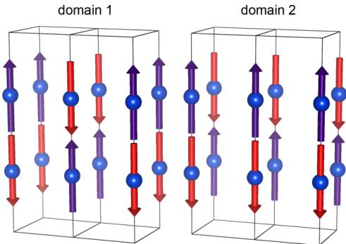
measurements and therefore we conclude that there exist two magnetic k domains, corresponding to the propagation vectors \( \mathbf{k} = (1/2,0,0) \) and k' = (0,1/2,0). These domains are equally populated. The resulting magnetic structure is depicted in Fig. 3.
Figure 4 shows the temperature dependence of the \( (1/2\ 0\ 1) \) magnetic reflection. Transition temperature \( T_{1}=10.4(2) \) K was determined from the inflection point of this dependence. It is in agreement with the value determined from specific heat [13] and is plotted in the phase diagram in Fig. 1.
Because the other members of the “218” compounds reveal \( k_{218} = (1/2, 1/2, 1/2) \) [20], \( Ho_{2}RhIn_{8} \) is the first member of this series with magnetic domains. Its structure is much more similar to the “115” compounds, revealing the identical

FIG. 3. (Color online) Magnetic structure of \( Ho_{2}RhIn_{8} \) in the AF1 phase. Two magnetic domains are shown. Orientation is the same as in Fig. 2.

FIG. 4. (Color online) Temperature dependence of integrated intensity of \( (1/2\ 0\ 1) \) reflection in different magnetic fields. Inset shows the intensity of the \( (1/2\ 0\ 1) \) reflection attributed to the AF1 phase (circles) together with \( (1/2\ 0.036\ 1) \) reflection attributed to the AF3 phase (squares). Lines are only to guide the eye.
stacking along the c axis and also the same propagation within the ab plane.
B. Field-induced structure AF2
In order to determine magnetic structure in the field-induced magnetic phase AF2, neutron diffraction experiments were carried out in the horizontal and vertical magnet in a field of 4 T. A thorough search in the reciprocal space leads to observation of magnetic reflections described by six propagation vectors: \( \mathbf{k}_{0} = (0,0,0) \) , \( \mathbf{k}_{1} = (1/2,0,0) \) , \( \mathbf{k}_{1}^{\prime} = (0,1/2,0) \) , \( \mathbf{k}_{2} = (1/2,0,1/2) \) , \( \mathbf{k}_{2}^{\prime} = (0,1/2,1/2) \) , and \( \mathbf{k}_{3} = (1/2,1/2,1/2) \) , where \( k_{1,2} \) and \( k_{1,2}^{\prime} \) correspond to different magnetic domains. Reciprocal space positions (1/2, 1/2, 0), (1/2, 3/2, 0), (1, 1, 1/2), and (1, 0, 1/2) were measured for a longer time, however, no magnetic reflections were found. The magnetic unit cell size is thus 2a, 2b, 2c. The sum of the magnetic moments associated with \( k_{1} \) , \( k_{2} \) , and \( k_{3} \) within the magnetic unit cell is always zero, as they are always propagating within the ab plane canceling out moments at the 2g Wyckoff site. The magnetization measurement clearly shows that the overall magnetic moment in the AF2 phase amounts to the half of the magnetic moment of Ho in ferromagnetic state above 6 T ( \( \approx 4 \mu_{B} \) ) [13]. This moment does not propagate and is associated with the ferromagnetic component ( \( k_{0} \) ) of the AF2 phase. Refinement of the measured ferromagnetic intensities using the FULLPROF software confirms this prediction and leads to the magnetic moment \( \mu_{k_{0}} = 3.6(4)\mu_{B} \) in agreement with magnetization measurements.
We have performed symmetry analysis based on representations theory for the remaining propagation wave vectors similarly to AF1. Possible directions of the magnetic moments are summarized in Table II. For structures with \( k_{1} \) and \( k_{2} \) there exist six allowed 1D irreducible representations. In case of \( k_{3} \) , there is a general possibility for the moment to lie in any direction within the ab plane (detailed symmetry and magnetic group analysis for this structure and propagation is discussed in Ref. [20]). Taking into account the fact that all moments in AF1 point along the c axis and that a clear field-induced spin-flip behavior is observed, we consider that magnetic moments associated with every wave vector k in AF2 point also along the c axis.
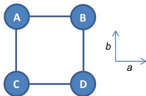
In order to construct possible magnetic structures, we will now focus on the magnetic spin arrangement within the \( (00z_{\mathrm{Ho}}) \) plane (highlighted in red in Fig. 2). This consideration simplifies the problem to two dimensions. There are four magnetic positions within this plane in the magnetic unit cell (marked A–D in Fig. 2), all corresponding to one atom site in the nuclear unit cell. There can exist four propagation vectors in maximum: \( \mathbf{k}_{0, \mathrm{plane}} = (0,0) \) , \( \mathbf{k}_{1, \mathrm{plane}} = (1/2,0) \) , \( \mathbf{k}_{2, \mathrm{plane}} = (0,1/2) \) , and \( \mathbf{k}_{3, \mathrm{plane}} = (1/2,1/2) \) . Considering only the spin-flip scenario, the total magnetic moments on all four sites \( \mu_{A-D} \) have necessarily the same amplitude. If we neglect the change of the magnitude of the magnetic moment and assume that the magnetic moments are along the c axis, the only possible solution exists:
\[ \mu_{\mathbf{k}_{0}}=\mu_{\mathbf{k}_{1}}=-\mu_{\mathbf{k}_{2}}=\mu_{\mathbf{k}_{3}}, \quad (1) \]
\[ \mu_{A}=-\mu_{B}=\mu_{C}=\mu_{D}=2\mu_{\mathbf{k}_{0}}. \quad (2) \]
In other words, the component associated with \( k_{2} \) has an opposite sign with respect to all other components and one of the four magnetic moments within the plane is flipped. For details of the derivation, see Appendix A.
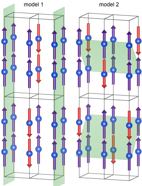
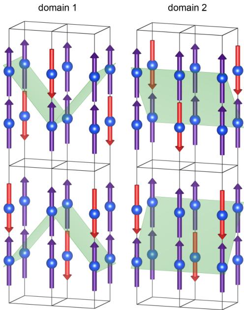
Extending from the 2D case to the real \( Ho_{2}RhIn_{8} \) structure brings more options (six propagation vectors, each with two possible stackings along the c axis). Taking into account the fact that the total magnetic moment at one site cannot be bigger than full magnetic moment of \( \mathrm{Ho}\left(10\mu_{B}\right) \) and \( \mu_{k_{0}} = 3.6(4)\mu_{b} \) , only two independent models summarized in Table III and depicted in Fig. 5 are possible. They are distinguishable on the same principle as in the case of the AF1 phase—on the basis of the existence of the reflections (hk0) for propagation vector \( k_{1} \) . These reflections are forbidden in the model 2. As we indeed did not observe any of these reflections, the correct model describing the magnetic structure of \( Ho_{2}RhIn_{8} \) in the AF2 phase is the model 2. Similarly to AF1, there exist two magnetic k domains. The resulting magnetic structure is shown in Fig. 6.
Quantitative refinement using the FULLPROF software confirmed described results and led to the magnetic moments associated with different propagation vectors as follows: \( \mu_{\mathbf{k}_{0}} = 3.6(4)\mu_{B} \) , \( \mu_{\mathbf{k}_{1}} = 3.7(3)\mu_{B} \) , and \( \mu_{\mathbf{k}_{2}} = -4.0(2)\mu_{B} \) . The amplitude of the magnetic moments described by the propaga-
TABLE III. Possible magnetic structures in the AF2 phase based on the propagation vectors analysis. Stacking along the c axis has the same meaning as in Table II.
| c axis stacking on site A (see Fig. 2) | ||
| Model 1 | Model 2 | |
| \( \mathbf{k}_{0} = (0, 0, 0) \) | +++ | +++ |
| \( \mathbf{k}_{1} = (1/2, 0, 0) \) | +++ | +-+ |
| \( \mathbf{k}_{2} = (0, 1/2, 1/2) \) | --++ | +-+ |
| \( \mathbf{k}_{3} = (1/2, 1/2, 1/2) \) | ++-- | ++-- |
| Overall stacking | +++ | +++- |

FIG. 5. (Color online) Possible magnetic structures in the AF2 phase with highlighted ferromagnetically ordered planes. Model 1 consists of ferromagnetic and antiferromagnetic (00l) planes. Model 2 is more complicated revealing ferromagnetically ordered atoms in some kind of zigzag planes. Orientation is the same as in Fig. 2.
tion vector \( k_{3} \) was not possible to determine, since due to the construction of magnets, we have reached only one magnetic reflection associated with this propagation. Reliability factors of the fitting procedure are stated in Table V in Appendix B. All three determined amplitudes satisfy Eq. (1) within their errors. The overall amplitude of magnetic moments is \( \mu_{AF2} = 7.5(5)\mu_{B} \) , which is calculated from Eq. (2) taking \( \mu_{k_{0}} \) as the mean of all three refined amplitudes of magnetic moments. The value of \( \mu_{AF2} \) is slightly bigger than \( \mu_{AF1} \) . This increase is due to the impact of the 4 T external magnetic field and is in agreement with the measured magnetization curves [13].
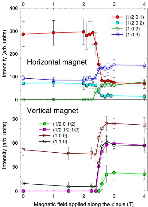
To clarify the location of the phase boundaries and verify consistency of the data from vertical and horizontal magnet, several reflections were followed with the changing magnetic field (Fig. 7). The transition from the AF1 to the AF2 phase is illustrated by a strong decrease of intensity of the \( (1/2\ 0\ 1) \) and \( (1/2\ 0\ 2) \) reflections together with increase of the intensity at the positions of the nuclear peaks and peaks described by the propagation vectors \( k_{2} \) and \( k_{3} \) . Temperature dependence of the \( (1/2\ 0\ 1) \) reflection in the fields of 2 T and 3 T is depicted in Fig. 4. The shape of the curve in 0 T and 2 T corresponds to each other showing the same ordering mechanism as both are entering the AF1 phase. The emergence of the AF1 phase within a limited temperature range in the field of 3 T, indicated by bulk measurements (Fig. 1), was not observed. This can

FIG. 6. (Color online) The magnetic structure of \( Ho_{2}RhIn_{8} \) in the AF2 phase. Two magnetic domains are equally populated. The orientation is the same as in Fig. 2.
be explained by the absence of a long-range order in the narrow AF1 phase region just below the ordering temperature in 3 T. Points from the measured temperature and the field dependencies are included in the phase diagram in Fig. 1.
The AF2 phase in \( Ho_{2}RhIn_{8} \) is the first solved field-induced magnetic structure within the \( R_{2}TIn_{8} \) and \( RTIn_{5} \) family preventing us from comparisons with related compounds. We suppose that, due to the similar phase diagrams, related compounds from the “218” family reveal the same flipping mechanism during metamagnetic transition from AF1 to AF2, consisting of the flip of 1/4 of the magnetic moments. The same assumption could be applied with a small modification to the “115” compounds, as the AF1 structure in \( Ho_{2}RhIn_{8} \) is very similar to the known “115” magnetic structures. On the basis of the magnetization measurements, Hieu suggested several possible magnetic structures in AF2 phase for “115” compounds [18]. One of these magnetic structures (Fig. 5.69(c) in Ref. [18]) corresponds to the model determined for the AF2 phase in \( Ho_{2}RhIn_{8} \) .
C. Incommensurate structure AF3
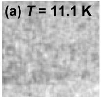
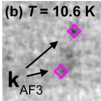
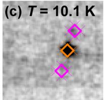
Magnetic intensity in the AF3 phase is illustrated in Fig. 8, which shows the identical detail of the Laue diagrams taken at different temperatures. At 11.1 K, above the Néel temperature, there is no significant intensity. At 10.6 K, two satellites at incommensurate position appear together with a very weak trace of a commensurate (1/2 0 1) reflection. The intensity

FIG. 7. (Color online) Field dependence of selected Bragg reflections in horizontal and vertical magnetic fields. Lines are there only to guide the eye.
of the commensurate reflection starts to grow and at 10.1 K there are clearly both commensurate and incommensurate reflections visible. The AF3 phase completely vanishes at


FIG. 8. (Color online) Detail of the region in the vicinity of \( (0.5\ 0\ 1) \) reflection in the Laue pattern taken at different temperatures.

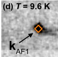
FIG. 9. (Color online) Cuts along the 0h0 crystallographic direction at different temperatures.
9.6 K. Integrated cut along the curves going through all three reflections are shown in Fig. 9. The same behavior was observed also around other strong magnetic reflections and the magnetic peaks on the incommensurate positions were indexed with the propagation vector \( \mathbf{k}_{AF3} = (1/2, \delta, 0) \) , where \( \delta = 0.036(3) \) . However, as the Laue patterns were taken during temperature sweep and all spots are well localized in reciprocal space at constant positions, \( \delta \) is temperature independent. This can be also seen in Fig. 9. The data are consistent with \( T_{N} = 10.9 \) K determined from specific heat measurements [13].
Formation of the incommensurate zero-field phase is unique within “218” and “115” compounds, but it can be found in the tetragonal compounds structurally related to the other well known heavy fermion superconductor \( CeCu_{2}Si_{2} \) (e.g., in \( UCu_{2}Si_{2} \) [29]). A tiny value of the incommensurate component of the propagation vector implicates modulation period involving about 27 holmium atoms. Such a long modulation can be explained by formation of a spin-density-wave phase.
D. Crystalline electric field
In order to understand the anisotropy in \( Ho_{2}RhIn_{8} \) , we have measured temperature dependence of the magnetic

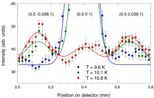
FIG. 10. (Color online) Temperature dependence of magnetic susceptibility (right axis) and inverse magnetic susceptibility (left axis) of \( Ho_{2}RhIn_{8} \) . Values are given per one mole, thus two Ho atoms. Solid line represents CEF fit of inverse susceptibility data.
TABLE IV. Summary of parameters obtained from the fit to Eq. (3) and determined crystal field parameters [Eq. (C2)].
| \( \chi_{0} \) (emu/mol) | \( \theta_{p} \) (K) | \( \mu_{\text{eff}} \) ( \( \mu_{B} \) ) | \( \lambda \) (mol/emu) | \( J_{\text{ex}} \) (K) | |
| [100] | 2.1(1) \( \times \) 10 \( ^{-3} \) | -21.1(1) | 10.08(2) | -1.31 | -0.68 |
| [001] | 0.5(1) \( \times \) 10 \( ^{-3} \) | -8.9(2) | 10.57(2) | -0.58 | -0.78 |
| \( B_{2}^{0} \) (K) | \( B_{4}^{0} \) (K) | \( B_{4}^{4} \) (K) | \( B_{6}^{0} \) (K) | \( B_{6}^{4} \) (K) | |
| -0.173 | 1.08 \( \times \) 10 \( ^{-3} \) | -1.27 \( \times \) 10 \( ^{-2} \) | -3.35 \( \times \) 10 \( ^{-6} \) | 9.70 \( \times \) 10 \( ^{-6} \) |
susceptibility in the applied magnetic field of 1 T along the crystallographic a and c axis. Inverse susceptibility data in the paramagnetic region (30–300 K) were fitted to the modified Curie-Weiss law,
\[ \chi=\chi_{0}+\frac{C}{T-\theta_{p}}, \quad (3) \]
where \( \chi_{0} \) is temperature independent susceptibility, \( \theta_{p} \) is paramagnetic Curie temperature and the effective magnetic moment \( \mu_{eff} \) is related to Curie constant C. Measured data are shown in Fig. 10 and determined parameters for each field direction are summarized in Table IV. We observe expected magnetic anisotropy as difference between two measured field directions. The rapid decrease of the magnetic susceptibility below ordering temperature in field along [001] direction confirms antiferromagnetic ordering with Ho moments along the c axis.
Further analysis of susceptibility data was done by fitting to the CEF model proposed by Stevens and Hutchings [30]. Details of this procedure as well as all used formulas are described in Appendix C. Solid lines in Fig. 10 are the results of CEF calculations which reproduce well the measured data. The CEF parameters and molecular field coefficients \( \lambda \) are summarized in Table IV. Calculated second-order parameter \( B_{2}^{0} \) is clearly dominant, in agreement with related \( RRhIn_{5} \) [14] and \( R_{2}CoGa_{8} \) [17] compounds. It is reported for both series, that sign of \( B_{2}^{0} \) parameter determines the easy magnetization axis. The change of the easy axis of magnetization takes place between Ho and Er compound within each series (discussed also in Ref. [15]). This can be understood by change of the sign of Stevens multiplication factor \( \alpha_{J} \) for rare-earth ions, because \( B_{2}^{0} \) is defined as \( A_{2}^{0}(r^{2})\alpha_{J} \) . Here \( A_{2}^{0} \) is constant for identical structures and \( r^{2} \) is always positive. As stated at the end of Sec. III A, zero-field magnetic structure AF1 in \( Ho_{2}RhIn_{8} \) differs from magnetic structures in other \( R_{2}RhIn_{8} \) compounds. Moreover, it is also different from its cobalt-gallium analog \( Ho_{2}CoGa_{8} \) , which has magnetic moments propagating with wave vector k = (1/2, 1/2, 1/2) [22] in agreement with other rhodium-indium compounds. In fact, \( Ho_{2}RhIn_{8} \) is the only compound from the rich \( R_{n}T_{m}X_{3n+2m} \) family with magnetic moments pointing along the c axis and the propagation vector k = (1/2, 0, 0). Determined \( B_{2}^{0} = -0.17 \) K for \( Ho_{2}RhIn_{8} \) is smaller than values reported earlier for related \( HoRhIn_{5} \) (-0.33 K [14]) and \( Ho_{2}CoGa_{8} \) (-0.22 K [17]) and is closer to the zero, where the easy c axis switches to the easy ab plane. Competing c and ab easy axis/planes in \( Ho_{2}RhIn_{8} \) can stand behind the unique anisotropic propagation within the ab plane and also existence of the zero-field incommensurate phase AF3. We have calculated exchange interaction \( J_{ex} \) according to the mean-field theory by using the same formulas as in Ref. [17]. The determined values are presented in Table IV. Both exchange constants are negative confirming antiferromagnetic interaction, but they are significantly increased in comparison with \( Ho_{2}CoGa_{8} \) [17]. This effect is reflected in the higher ordering temperature of \( Ho_{2}RhIn_{8} \) .
IV. CONCLUSION
We have determined the magnetic structures in \( Ho_{2}RhIn_{8} \) by means of neutron diffraction experiments. In the zero-field ordered state, the magnetic order is characterized by a single propagation vector \( \mathbf{k}_{AF1} = (1/2, 0, 0) \) with the antiferromagnetic coupling of Ho moments along the c axis and the amplitude of the magnetic moment \( 6.9(2)\mu_{B} \) . Before entering this ground-state commensurate phase, there exists a small temperature region where the incommensurate phase with propagation \( \mathbf{k}_{AF3} = (1/2, 0.036, 0) \) develops. Both existence of the additional incommensurate phase and the ground-state propagation vector anisotropic within ab plane are unique within the \( R_{n}T_{m}X_{3n+2m} \) series. Analysis of the temperature dependence of magnetic susceptibility revealed paramagnetic Curie temperatures and set of crystal field parameters, which are in agreement with observed anisotropic magnetic structures. These results confirm that magnetism in \( Ho_{2}RhIn_{8} \) is purely CEF driven. The mean-field theory model can be used for the estimation of the magnetic exchange constants and magnetic structures.
In the applied magnetic field along the c axis the magnetic structure transforms by spin flipping of the 1/4 of magnetic moments to another commensurate phase with the amplitude of magnetic moment \( 7.5(5)\mu_{B} \) (in B = 4 T). Similar flipping behavior is expected also in the other related compounds with the same phase diagram.
ACKNOWLEDGMENTS
This work was supported by the Czech Science Foundation under Grant No. P204-13-12227S. The work is a part of research project LG14037 financed by the Ministry of Education, Youth and Sports, Czech Republic. Sample preparation and bulk measurements were carried out in MLTL (http://mltl.eu/), which also is supported by the Ministry of Education, Youth and Sports, Czech Republic within the program of Czech Research Infrastructures (Project No. LM2011025). This project has received funding from the European Union's Seventh Framework Programme for research, technological development and demonstration under the NMI3-II Grant No. 283883. We thank HZB and ILL for the allocation of neutron beamtimes.

FIG. 11. (Color online) Schematic view on Ho atoms in ab plane of magnetic unit cell. Each atom position is marked with a letter.
APPENDIX A: MAGNETIC STRUCTURE DERIVATION
Generally, moment distribution \( \mu_{j} \) associated with the atom j of a magnetic structure can be Fourier expanded according to:
\[ \mu_{j}=\sum_{\{\mathbf{k}\}}\Psi_{\mathbf{k}}^{j}e^{-2\pi i\mathbf{k}\cdot\mathbf{T}}, \quad (A1) \]
where \( \Psi_{\mathbf{k}}^{j} \) is the basis vector associated with the propagation vector k and the atom on the position j and T is the corresponding lattice translation vector. The summation is made over all wave vectors that are confined to the first Brillouin zone. If we neglect the change of the magnitude of the magnetic moment and assume that the magnetic moments lie along the c axis, Eq. (A1) will simplify to:
\[ \mu_{j}=\sum_{\{\mathbf{k}\}}\mu_{\mathbf{k}}\cos(\mathbf{k}\cdot\mathbf{T}), \quad (A2) \]
where cosine has always maximal amplitude.
We will now focus on the magnetic spin arrangement within \( 2a \times 2b \) plane, where there are four magnetic positions in the magnetic unit cell (marked A–D in Fig. 11), all corresponding to one atom site in the nuclear unit cell. There exist four propagation vectors in maximum: \( \mathbf{k}_{0, \text{plane}} = (0,0) \) , \( \mathbf{k}_{1, \text{plane}} = (1/2,0) \) , \( \mathbf{k}_{2, \text{plane}} = (0,1/2) \) , and \( \mathbf{k}_{3, \text{plane}} = (1/2,1/2) \) . In the following text, the subscript plane will be omitted for better readability. Regarding Eq. (A2), total magnetic moments on A–D sites can be calculated as:
\[ \mu_{A}=\mu_{\mathbf{k}_{0}}+\mu_{\mathbf{k}_{1}}+\mu_{\mathbf{k}_{2}}+\mu_{\mathbf{k}_{3}}, \quad (A3) \]
\[ \mu_{B}=\mu_{\mathbf{k}_{0}}-\mu_{\mathbf{k}_{1}}+\mu_{\mathbf{k}_{2}}-\mu_{\mathbf{k}_{3}}, \quad (A4) \]
\[ \mu_{C}=\mu_{\mathbf{k}_{0}}+\mu_{\mathbf{k}_{1}}-\mu_{\mathbf{k}_{2}}-\mu_{\mathbf{k}_{3}}, \quad (A5) \]
\[ \mu_{D}=\mu_{\mathbf{k}_{0}}-\mu_{\mathbf{k}_{1}}-\mu_{\mathbf{k}_{2}}+\mu_{\mathbf{k}_{3}}. \quad (A6) \]
Considering the spin-flip ratio only, the total magnetic moments on all four sites must have the same amplitude:
\[ |\mu_{A}|=|\mu_{B}|=|\mu_{C}|=|\mu_{D}|, \quad (A7) \]
Now we will reduce Eqs. (A3)–(A6) using (A7). By combining (A3) and (A4):
\[ \mu_{\mathbf{k}_{0}}=-\mu_{\mathbf{k}_{2}}\quad\mathrm{o r}\quad\mu_{\mathbf{k}_{1}}=-\mu_{\mathbf{k}_{3}}. \quad (A8) \]
By combining (A3) and (A5):
\[ \mu_{\mathbf{k}_{2}}=-\mu_{\mathbf{k}_{3}}\quad\mathrm{o r}\quad\mu_{\mathbf{k}_{1}}=-\mu_{\mathbf{k_{2}}}. \quad (A9) \]
By combining (A3) and (A6):
\[ \mu_{\mathbf{k}_{1}}=-\mu_{\mathbf{k}_{2}}\quad\mathrm{o r}\quad\mu_{\mathbf{k_{0}}}=-\mu_{\mathbf{k_{3}}}. \quad (A10) \]
We have three sets of equations (A8)–(A10), each with two alternatives—that is together eight combinations. Only four of them are not in contradiction with each other and result in:
\[ -\mu_{\mathbf{k}_{0}}=\mu_{\mathbf{k}_{1}}=\mu_{\mathbf{k}_{2}}=\mu_{\mathbf{k}_{3}}, \quad (A11) \]
\[ \mu_{\mathbf{k}_{0}}=-\mu_{\mathbf{k}_{1}}=\mu_{\mathbf{k}_{2}}=\mu_{\mathbf{k}_{5}}, \quad (A12) \]
\[ \mu_{\mathbf{k}_{0}}=\mu_{\mathbf{k}_{1}}=-\mu_{\mathbf{k}_{2}}=\mu_{\mathbf{k}_{3}}, \quad (A13) \]
\[ \mu_{\mathbf{k}_{0}}=\mu_{\mathbf{k}_{1}}=\mu_{\mathbf{k}_{5}}=-\mu_{\mathbf{k}_{3}}. \quad (A14) \]
This means that one of the moments associated with propagation vectors is always flipped. Using Eqs. (A3)–(A6), one will get:
\[ -\mu_{A}=\mu_{B}=\mu_{C}=\mu_{D}=2\mu_{\mathbf{k}_{0}}, \quad (A15) \]
\[ \mu_{A}=-\mu_{B}=\mu_{C}=\mu_{D}=2\mu_{\mathbf{k}_{0}}. \quad (A16) \]
\[ \mu_{A}=\mu_{B}=-\mu_{C}=\mu_{D}=2\mu_{\mathbf{k}_{0}}, \quad (17) \]
\[ \mu_{A}=\mu_{B}=\mu_{C}=-\mu_{D}=2\mu_{\mathbf{k}_{0}}. \quad (A18) \]
Equations (A15)–(A18) are analogical because of the crystal symmetry. This means that one of the moments within the magnetic unit cell is always flipped. For the consideration in the paper, we have chosen Eq. (A16).
APPENDIX B: RELIABILITY FACTORS
We present results of the FULLPROF data treatment of magnetic structures in the AF1 and AF2 phase in \( Ho_{2}RhIn_{8} \) . Refinement was not possible for propagation vector \( k_{1} \) in vertical magnet, because all measured reflections were forbidden. It could not be performed for the propagation vector \( k_{3} \) either, because only one reflection was reachable with this propagation. Determined magnetic moments for all phases together with the reliability factors are stated in Table V.
TABLE V. Summary of FULLPROF treatment of the measured reflections in \( Ho_{2}RhIn_{8} \) .
| Phase | AF1 | AF2 | ||||||
| Type of magnet | - | hor. | hor. | ver. | ver. | ver. | ver. | ver. |
| Propagation vector | k | k0 | k1 | k0 | k1 | k2 | k3 | |
| Number of reflections | 7 | 7 | 7 | 3 | 16 | 16 | 1 | |
| Magnetic moment \( \mu_{\mathrm{k}} \) ( \( \mu_{B} \) ) | 6.9(2) | 3.5(2) | 3.7(2) | 3.8(6) | - | 4.0(2) | - | |
| \( RF^{2} \) | 17.0 | 81.7 | 9.37 | 40.4 | - | 22.8 | - | |
| RF | 7.91 | 44.0 | 5.26 | 21.6 | - | 11.9 | - | |
| \( \chi \) | 0.53 | 2.09 | 0.14 | 2.86 | - | 1.06 | - |
APPENDIX C: CRYSTAL FIELD DATA TREATMENT
Holmium ions occupy sites with tetragonal symmetry, which simplifies CEF Hamiltonian to only five independent parameters:
\[ \mathcal{H}_{\mathrm{C E F}}=B_{0}^{2}O_{0}^{2}+B_{0}^{4}O_{0}^{4}+B_{4}^{4}O_{4}^{4}+B_{6}^{0}O_{6}^{0}+B_{6}^{4}O_{6}^{4}, \quad (C1) \]
where \( B_{l}^{m} \) are CEF parameters and \( O_{l}^{m} \) are Stevens operators [30]. Magnetic susceptibility \( \chi \) includes CEF susceptibility \( \chi_{CEF} \) , the molecular field contribution \( \lambda \) and already determined \( \chi_{0} \) :
\[ \chi=\frac{1}{\chi_{\mathrm{CEF}}^{-1}-\lambda}+\chi_{0}, \quad (C2) \]
[1] J. Thompson, R. Movshovich, Z. Fisk, F. Bouquet, N. Curro, R. Fisher, P. Hammel, H. Hegger, M. Hundley, M. Jaime, P. Pagliuso, C. Petrovic, N. Phillips, and J. Sarrao, J. Magn. Magn. Mater. 226–230, 5 (2001).
[2] C. Pfleiderer, Rev. Mod. Phys. 81, 1551 (2009).
[3] Q. Si, Physica B (Amsterdam) 378–380, 23 (2006).
[4] J. Custers, K. Lorenzer, M. Müller, A. Prokofiev, A. Sidorenko, H. Winkler, A. Strydom, Y. Shimura, T. Sakakibara, R. Yu et al., Nature Mater. 11, 189 (2012).
[5] M. Nicklas, V. A. Sidorov, H. A. Borges, P. G. Pagliuso, C. Petrovic, Z. Fisk, J. L. Sarrao, and J. D. Thompson, Phys. Rev. B 67, 020506 (2003).
[6] D. Kaczorowski, A. P. Pikul, D. Gnida, and V. H. Tran, Phys. Rev. Lett. 103, 027003 (2009).
[7] K. Uhliřová, J. Prokleška, and V. Sechovský, Phys. Rev. Lett. 104, 059701 (2010).
[8] C. Petrovic, P. G. Pagliuso, M. F. Hundley, R. Movshovich, J. L. Sarrao, J. D. Thompson, Z. Fisk, and P. Monthoux, J. Phys. Condens. Matter 13, L337 (2001).
[9] W. Bao, P. G. Pagliuso, J. L. Sarrao, J. D. Thompson, Z. Fisk, J. W. Lynn, and R. W. Ervin, Phys. Rev. B 62, R14621 (2000).
[10] E. D. Bauer, H. O. Lee, V. A. Sidorov, N. Kurita, K. Gofryk, J.-X. Zhu, F. Ronning, R. Movshovich, J. D. Thompson, and T. Park, Phys. Rev. B 81, 180507 (2010).
[11] A. Tursina, S. Nesterenko, Y. Seropegin, H. N. 1, and D. Kaczorowski, J. Solid State Chem. 200, 7 (2013).
[12] M. Kratochvílová, M. Dušek, K. Uhliřová, A. Rudajevová, J. Prokleška, B. Vondráčková, J. Custers, and V. Sechovský, J. Cryst. Growth 397, 47 (2014).
[13] P. Čermák, M. Kratochvílová, K. Pajskr, and P. Javorský, J. Phys. Condens. Matter 24, 206005 (2012).
[14] N. V. Hieu, T. Takeuchi, H. Shishido, C. Tonohiro, T. Yamada, H. Nakashima, K. Sugiyama, R. Settai, T. D. Matsuda, Y. Haga, M. Hagiwara, K. Kindo, S. Araki, Y. Nozue, and Y. Ōnuki, J. Phys. Soc. Jpn. 76, 064702 (2007).
where \( \chi_{CEF} \) is given by
\[ \chi_{\mathrm{CEF}}=N(g_{J}\mu_{\mathrm{B}})^{2}e^{\frac{E_{n}}{k_{\mathrm{B}}T}}\left(\sum_{m\neq n}|\langle m|J|n\rangle|^{2}\frac{1-e^{-\frac{\Delta_{m,n}}{k_{\mathrm{B}}T}}}{\Delta_{m,n}}e^{-\frac{E_{n}}{k_{\mathrm{B}}T}}\right. \]
\[ +\frac{1}{k_{\mathrm{B}}T}\sum_{n}|\langle n|J|n\rangle|^{2}e^{-\frac{E_{n}}{k_{\mathrm{B}}T}}\Bigg), \quad (C3) \]
where \( g_{J} \) is the Landé g factor, J is the component of the angular momentum in direction of applied magnetic field and \( \Delta_{m,n} = E_{n} - E_{m} \) .
Experimental data in the whole temperature range were fitted with Eq. (C2) using nonlinear optimization algorithm called generalized reduced gradient (GRG2) [31]. We have used randomly selected starting parameters and run the method more than 1000 times to find not only local, but also global minima.
[15] J. Hudis, R. Hu, C. Broholm, V. Mitrovi, and C. Petrovic, J. Magn. Magn. Mater. 307, 301 (2006).
[16] P. Javorský, K. Pajskr, M. Klicpera, P. Čermák, Y. Skourski, and A. Andreev, J. Alloys Compd. 598, 278 (2014).
[17] D. A. Joshi, R. Nagalakshmi, S. K. Dhar, and A. Thamizhavel, Phys. Rev. B 77, 174420 (2008).
[18] N. V. Hieu, Ph.D. thesis, Osaka University, 2007.
[19] R. Kobayashi, K. Kaneko, S. Wakimoto, S. Chi, N. Sanada, R. Watanuki, and K. Suzuki, J. Korean Phys. Soc. 63, 337 (2013).
[20] P. Čermák, P. Javorský, M. Kratochvílová, K. Pajskr, M. Klicpera, B. Ouladdiaf, M.-H. Lemée-Cailleau, J. Rodriguez-Carvajal, and M. Boehm, Phys. Rev. B 89, 184409 (2014).
[21] J. R. L. Mardegan, C. Adriano, R. F. C. Vescovi, G. A. Faria, P. G. Pagliuso, and C. Giles, Phys. Rev. B 89, 115103 (2014).
[22] C. Adriano, C. Giles, L. Coelho, G. Faria, and P. Pagliuso, Physica B (Amsterdam) 404, 3289 (2009).
[23] B. Ouladdiaf, J. Archer, J. R. Allibon, P. Decarpentrie, M.-H. Lemée-Cailleau, J. Rodríguez-Carvajal, A. W. Hewat, S. York, D. Brau, and G. J. McIntyre, J. Appl. Crystallogr. 44, 392 (2011).
[24] J. Rodriguez-Carvajal, L. Fuentes-Montero, and P. Čermák, http://lauescite.com/.
[25] C. Wilkinson, H. Khamis, R. Stansfield, and G. McIntyre, J. Appl. Crystallogr. 21, 471 (1988), see https://forge.ep-campus.eu/projects/sxtalsoft/repository/show/racer.
[26] J. Rodriguez-Carvajal, Physica B 192, 55 (1993), the complete FULLPROF suite of programs can be obtained from: https://www.ill.eu/sites/fullprof.
[27] W. Zachariasen, Acta Crystallogr. 23, 558 (1967).
[28] J. Rodriguez-Carvajal, see https://www.ill.eu/sites/fullprof/php/Fullprof_News_2002.htm.
[29] F. Honda, N. Metoki, T. D. Matsuda, Y. Haga, and Y. Onuki, J. Phys. Condens. Matter 18, 479 (2006).
[30] M. T. Hutchings, Solid State Phys. 16, 227 (1964).
[31] L. S. Lasdon, A. D. Waren, A. Jain, and M. Ratner, ACM Trans. Math. Softw. 4, 34 (1978).
 p2_0.jpg
 p3_0.jpg
 p3_1.jpg
 p4_0.jpg
 p5_0.jpg
 p5_1.jpg
 p6_0.jpg
 p6_1.jpg
 p6_2.jpg
 p6_3.jpg
 p6_4.jpg
 p6_5.jpg
 p6_6.jpg
 p8_0.jpg