NpS (3.9)
Three+ propagation vectors| Transition Temperature | 23 K |
|---|---|
| Parent Space Group | Fm-3m (#225) |
| Magnetic Space Group | FSd-3c (#228.139) |
| Magnetic Point Group | m-3m1' (32.2.119) |
| Lattice Parameters | 11.05400 11.05400 11.05400 90.00 90.00 90.00 |
|---|---|
| DOI | 10.1016/0921-4526(95)00021-z |
| Reference | G. Lander and P. Burlet, Physica B: Condensed Matter (1995) 215 7-21. |
| Label | Element | Mx | My | Mz | |M| |
|---|---|---|---|---|---|
| Np1 | Np | 0.4 | 0.4 | 0.4 | 0.69 |
Title
On the magnetic structure of actinide monopnictides
Authors
G.H. Lander \( ^{a,*} \) P. Burlet \( ^{b} \) \( ^{a} \) European Commission, JRC, Institute for Transuranium Elements, Postfach 2340, D-76125 Karlsruhe, Germany \( ^{b} \) CEA-Département de la Recherche Fondamentale sur la Matière Condensée, SPSMS, MDN, 85X, 38045 Grenoble Cedex, France
Materials Studied
The paper primarily reviews the magnetic structures of actinide monopnictides (AnX) and monochalcogenides (AnZ), which have the FCC NaCl crystal structure. Specific materials discussed and listed in Table 1 include: * Uranium compounds: UN, UP, UAs, USb, UBi, US, USe, UTe * Neptunium compounds: NpN, NpP, NpAs, NpSb, NpBi, NpS, NpSe, NpTe * Plutonium compounds: PuN, PuP, PuAs, PuSb, PuBi, PuS, PuSe, PuTe * Solid solutions and mixed systems: UP-US, UAs-US, UAs$_{1-x}$S$_{x}$, USb-UTe, U$_{0.85}$Th$_{0.15}$Sb, USb$_{0.8}$Te$_{0.2}$, NpAs$_{0.95}$Se$_{0.05}$ * Other actinide compounds mentioned for comparison: UO$_{2}$, URu$_{2}$Si$_{2}$ * Lanthanide compounds mentioned for comparison: CeSb, NdIn$_{3}$ * Transition metal compounds mentioned for comparison: MnO, (Fe,Ni)$_{3}$Mn
Key Information
-
Crystal Structure / Space Group: All actinide monopnictides and monochalcogenides discussed have the FCC NaCl crystal structure. (Space group not explicitly stated, but NaCl structure typically corresponds to Fm-3m).
-
Lattice Parameters (a at 300 K):
- UN: 4.890 Å
- UP: 5.589 Å
- UAs: 5.779 Å
- USb: 6.191 Å
- UBi: 6.364 Å
- NpN: 4.897 Å
- NpP: 5.615 Å
- NpAs: 5.838 Å
- NpSb: 6.254 Å
- NpBi: 6.438 Å
- PuN: 4.905 Å
- PuP: 5.550 Å
- PuAs: 5.780 Å
- PuSb: 6.240 Å
- PuBi: 6.350 Å
- US: 5.489 Å
- USe: 5.750 Å
- UTe: 6.155 Å
- NpS: 5.527 Å
- NpSe: 5.804 Å
- NpTe: 6.198 Å
- PuS: 5.536 Å
- PuSe: 5.775 Å
- PuTe: 6.151 Å
-
Magnetic Ordering Type and Temperature (T_N, T_C):
- UN: T_N = 53 K, 1k type I
- UP: T_N = 122 K (1k type I), T_N = 22 K (2k type I)
- UAs: T_N = 124 K (1k type I), T_N = 62 K (2k type IA)
- USb: T_N = 213 K, 3k type I
- UBi: T_N = 285 K, Type I
- NpN: T_C = 87 K, Ferro
- NpP: T_N = 130 K (3k, incomm), T_N = 74 K (1k, 3+, 3-)
- NpAs: T_N = 173 K (1k, incomm), T_N = 154 K (1k, 4+, 4-), T_N = 138 K (3k, type I)
- NpSb: T_N = 202 K, 3k, type I
- NpBi: T_N = 193 K, 3k, type I
- PuN: T_N = 13? K
- PuP: T_C = 126 K, Ferro
- PuAs: T_C = 125 K, Ferro
- PuSb: T_N = 85 K (1k, Inc), T_C = 70 K (Ferro)
- PuBi: T_N = 58 K (1k, comm)
- US: T_C = 170 K, Ferro
- USe: T_C = 160 K, Ferro
- UTe: T_C = 104 K, Ferro
- NpS: T_N = 23 K, 4k, type II
- NpSe: T
On the magnetic structure of actinide monopnictides
G.H. Lander \( ^{a,*} \) , P. Burlet \( ^{b} \)
\( ^{a} \) European Commission, JRC, Institute for Transuranium Elements, Postfach 2340, D-76125 Karlsruhe, Germany \( ^{b} \) CEA-Département de la Recherche Fondamentale sur la Matière Condensée, SPSMS, MDN, 85X, 38045 Grenoble Cedex, France
Received 4 July 1994
Abstract
The magnetic structures of the actinides (i.e. those materials containing 5f electrons) exhibit considerable complexity. The reasons for this are a competition between exchange, often anisotropic in nature, crystal-field, and quadrupolar interactions. Based on work on compounds of the lanthanides (4f electrons), we have well-developed mechanisms for understanding magnetic structures. The problem in the actinides is compounded by our inability to quantify the individual interactions. The reason for this difficulty is the hybridization that often occurs between the 5f electrons surrounding the actinide with both the conduction electrons and those of the surrounding atoms. To simplify this paper we shall discuss only one set of magnetic structures, those of the actinide monopnictides. These have received perhaps the most attention of any series, and exemplify the complexities and challenges of this field; one to which Jean Rossat-Mignod made seminal contributions.
1. Introduction
Investigations of magnetic structure are as central to magnetism as investigations of the crystal structure are to chemistry. Without knowing the magnetic structure, and its dependence on external variables (temperature T, magnetic field H, pressure P, and uniaxial stress \( \sigma \) ), one simply cannot interpret measurements of any property in the magnetic state. Prior to the exploitation of neutrons for magnetic structure determination, there was no technique capable of giving this vital information. This changed with the developments of neutron diffraction, and the first paper on MnO by Shull and Smart [1] in 1949. Neutrons have now been used to determine literally hundreds of magnetic structures, and will no doubt continue to do so – but, as we will indicate below, neutrons cannot always give the complete answer. The problem of understanding why a material develops a certain magnetic structure is actually more complex than determining the structure itself with today's neutron technology. Of course, understanding why a material resides in a particular crystal structure is equally as complex, but it does not stop the continuing determination of complex crystal structures. For magnetic structures there are certain guidelines which help us in this process. We shall concentrate in this article on the actinide monopnictides. These have the FCC NaCl crystal structure and form a large set. Determining and understanding their magnetic structures has been an activity spread over almost 30 years, and illustratates many of the challenges and difficulties in actinide research.
2. Historical development of the determination of the magnetic structures
The first determinations of the magnetic structures of all the UX compounds were performed on polycrystalline

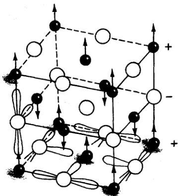
Fig. 1. Type-I magnetic structure of most of the UX compounds, uranium atoms are solid, pnictide atoms are open circles. The magnetic moments point along the axis of propagation of the magnetic structure. Schematically in this figure is also indicated the way in which the uranium 5f wave functions interact with the anion p wave functions in the plane perpendicular to the propagation direction (taken from Ref. [38]).
samples in the 1960s [2] in Harwell, Argonne, and Poland. The periodicities \( (k) \) of these structures were easy to establish – they are all commensurate – and in most cases correspond to a magnetic cell of the same size as the chemical unit cell \( (k=1) \) . The simple so-called type-I magnetic ordering is illustrated in Fig.1. These structures are characterized by ferromagnetic planes with a stacking + - + - . UAs was found to have a transition to a second structure at roughly \( T_{N}/2 \) to the structure with k=0.5, which corresponds to the stacking + + - - . This structure was first discovered in the UP-US solid solution [3] and was called (for no particular good reason except that types II, etc. are well-specified in FCC systems [4]) type-IA. It was known that these structures were longitudinal in nature because the \( (001) \) magnetic peak was absent, and this signifies (see Section 3) that the moments must lie parallel to the propagation direction.
Experiments on mixed systems, e.g. UP-US [5, 6] and UAs-US [7, 8] showed that the stacking arrangement of the ferromagnetic planes could be arranged in a variety of ways, e.g. \( 5 + , 4 - (k = 0.222) \) was found in \( UP_{0.75}S_{0.25} \) [6], and even incommensurate structures were found ( \( k = 0.36 \pm 0.01 \) ) in the \( UAs_{1-x}S_{x} \) [8] solid solution. A steady decrease of k was found across a system such as UP-US going from k = 1 in UP to k = 0 in US (a ferromagnet). This reinforced the idea that the conduction electrons were playing a key role through the RKKY coupling, an idea first advanced by Grunzweig-Genossar et al. [9] in what was the first major attempt to understand the properties of the UX compounds.
The first experiments on Np monopnictides [10] further emphasized the importance of the longitudinal magnetic structures, and showed that it was a general feature of the AnX (An = U, Np, Pu) compounds. Incommensurate magnetic structures were found in both NpP and NpAs – in both cases the structure locked into commensurate modulations as the temperature was lowered. This behavior is understood from energy considerations because the incommensurate structure has unequal moments on different atomic sites and this is not the lowest energy configuration [11]. It seemed by \( \sim \) 1974 that the magnetic structures of all the actinide monopnictides were reasonably well-understood; they were all longitudinal and the point of interest was in determining the value of k. The possibility that the structures might be more complicated and perhaps of the multi-k variety apparently did not occur to most people, especially the group at Argonne. Table 1 gives our present understanding of these structures.
In 1974 two important developments took place in this saga. First was the publication of a series of X-ray measurements on many of these compounds at low temperature \( [12] \) , and the second was the production of the first single crystal of USb at the ETH, Zürich by Vogt and Mattenberger \( [13] \) . The X-ray measurements showed that there was a difference between the ferromagnets \( (k=0) \) , which show a large lattice distortion below \( T_{C} \) , and the antiferromagnets \( (k>0) \) , many of which show no lattice distortion below \( T_{N} \) . Table 1 gives the values as known today. This difference between the ferro- and antiferromagnets seemed inexplicable on the basis of the simple longitudinal single-k structures then considered. The availability of single crystals of USb (UN single crystals had been available earlier \( [14] \) but the moment in UN is small) allowed detailed form-factor measurements to be undertaken \( [15] \) . These showed that the crystal-field ground state was such as to prefer a \( \langle111\rangle \) easy axis of magnetization, and yet the accepted view of the structure of USb (as in Fig. 1) was with the moments pointing along the cube directions, \( \langle001\rangle \) .
It was at this stage that Rossat entered the field. As usual, he was not about to accept 'conventional wisdom' and he set about with his usual vigor.
3. Neutron scattering and the multi-k magnetic structures
For a description of the fundamentals of the neutron scattering in the study of magnetic structures the Chapter written by Rossat-Mignod in 1986 [16] is an excellent
Table 1
Magnetic properties of U, Np, and Pu monopnictides and monochalcogenides \( ^{a} \)
| a(Å) (300 K) | T_{N} (K) | T_{C} (K) | k | Ordering | Easy axis | 10^{4} \times (c - a)/u (\pm 2) | \mu_{B}(T = 0) (\pm 0.05) | |
| UN | 4.890 | 53 | <001> | 1k type I | <001> | > 0? | 0.75 | |
| UP | 5.589 | 122 | <001> | 1k type I | <01> | \leq 5 | 1.7 | |
| 22 | <001> | 2k type I | <011> | \leq 5 | 1.9 | |||
| UAs | 5.779 | 124 | <001> | 1k type I | <00> | <0? | 1.9 | |
| 62 | <001/2> | 2k type IA | <011> | \sim + 2 | 2.25 | |||
| USb | 6.191 | 213 | <001> | 3k type I | <111> | < 2 | 2.85 | |
| UBi | 6.364 | 285 | <001> | Type I | ? | ? | 3.0 | |
| NpN | 4.897 | 87 | 0 | Ferro | <111> | (R) - 52 | 1.4 | |
| NpP | 5.615 | 130 | <000.36> | 3k, incomm | <001> | |||
| 74 | <001/3> | 1k, 3 + , 3 - | <001> | (T) - 42 | 2.2 | |||
| NpAs | 5.838 | 173 | <001/4-c> | 1k, incomm | <001> | |||
| 154 | <001/4> | 1k, 4 + , 4 - | <001> | (T) - 8 | \sim 2 | |||
| 138 | <001> | 3k, type I | <111> | < 3 | 2.5 | |||
| NpSb | 6.254 | 202 | <001> | 3k, type I | <<111> | < 15 | 2.5 | |
| NpBi | 6.438 | 193 | <001> | 3k, type I | <<111> | ? | 2.48 | |
| PuN | 4.905 | 13? | ||||||
| PuP | 5.550 | 126 | 0 | Ferro | <001> | (T) - 31 | 0.75 | |
| PuAs | 5.780 | 125 | 0 | Ferro | <001> | ? | 0.67 | |
| PuSb | 6.240 | 85 | <000.13> | 1k, Inc | <001> | ? | ||
| 70 | 0 | Ferro | <001> | ? | ||||
| PuBi | 6.350 | 58 | <000.23> | 1k, comm | <001> | ? | 0.50 | |
| US | 5.489 | 170 | 0 | Ferro | <111> | (R) + 105 | 1.70 | |
| USc | 5.750 | 160 | 0 | Ferro | <111> | (R) +81 | 2.0 | |
| UTc | 6.155 | 104 | 0 | Ferro | <111> | (R) +67 | 2.25 | |
| NpS | 5.527 | 23 | <1/2, 1/2, 1/2> | 4k, type II | <111> | < 3 | 0.7 | |
| NpSe | 5.804 | 38 | <1/2, 1/2, 1/2> | 4k, type II | <111> | ? | 1.3 | |
| NpTe | 6.198 | 40 | <1/2, 1/2, 1/2 | 4k, type II | <111> | ? | ||
| PuS | 5.536 | TIP | ||||||
| PuSe | 5.775 | TIP | ||||||
| PvTe | 6.151 | TIP |
\( ^{a} \) Note: Information is taken principally from Rossat-Mignod et al. (1984) \( ^{[2]} \) and Burlet et al. (1988) \( ^{[63]} \) and (1992) \( ^{[64]} \) . Comm. and incomm. refer to commensurate and incommensurate structures, respectively. TIP indicates temperature-independent paramagnetism. Recall that the crystallographic nomenclature \( \langle00\rangle1 \) indicates all six equivalent cube axis directions, etc. The distortions have been normalized with respect to the direction 'c' parallel to the moment direction, and 'a' perpendicular to it. Thus, in the cubic paramagnetic phase \( c/a=1 \) and the tetragonal distortion \( (T) \) simply changes these lengths. For a rhombohedral distortion \( (R) \) , the change from the rhombohedral angle of \( 60^{\circ} \) is given by \( \Delta x=-(4/\sqrt{27})\times(c-a)/a \) rad in the units used in the table.
reference. It is well-known that the elastic magnetic cross-section is proportional to the square of the component of the magnetic structure factor perpendicular to the scattering vector Q e.g. \( \left|F_{\mathbf{M},-}(\mathbf{Q})\right|^{2} \) . To obtain this structure factor we must identify the different Bravais lattices, their number \( n_{B} \) , and for each lattice j the moment distribution \( m_{n,j} \) can be Fourier expanded
\[ m_{n j}=\sum_{k}m_{k j}\exp(-\mathrm{i}\boldsymbol{k}\cdot\boldsymbol{R}_{n}). \quad (1) \]
The wave vectors k which enter the summation are confined within the first Brillouin zone. The structure factor is related to the Fourier components by
\[ F_{\mathbf{M}}(\mathbf{Q}=\mathbf{H}+\mathbf{k})=\left(\frac{\gamma e^{2}}{2m c^{2}}\right)\sum_{j}\mathbf{m}_{k,j}f_{j}(\mathbf{Q})\mathbf{e}^{\mathrm{i}\mathbf{Q}\cdot\mathbf{r}_{j}}\mathbf{e}^{-\mathbf{w}_{j}}. \quad (2) \]
The magnetic superlattice peaks associated with the wave vectors k are located in reciprocal points defined by the scattering vectors \( Q = H + k \) , where H defines the reciprocal lattice of the chemical unit cell. The observed intensity is proportional to the square of the structure factor. The initial term \( (\cdot)^{2} = 0.2696 \times 10^{-12} \) cm arises from the interaction between the neutron and the magnetic
moment of the electrons, the form factor \( f_{j}(\mathbf{Q}) \) refers to the spatial extent of the magnetic electrons [2, 17], and the term \( e^{-W} \) is the Debye-Waller factor. In this article we shall not discuss further either the form factor or the Debye-Waller factor. The latter is negligible in metallic systems at low temperature. There will, of course, be a number of k vectors that are equivalent; these are deduced by the symmetry operations of the paramagnetic space group. The set of wave vectors \( \{k\} \) is called the star of k and contains an even number of vectors because \( \pm k \) and \( \mp k \) are equivalent.
In practice, the first task is to determine k. This can often best be done with polycrystalline samples because they look at all reciprocal space, and this was done, as we have discussed, in the 1960s for the UX compounds. The second step is to measure the intensities to understand the coupling and also the direction of the moments. Here, again, the task is deceptively simple in the AnX systems. Reciprocal lattice points such as \( (100, (0\ 1\ 0) \) , and \( (00\ 1) \) have zero intensity. Given that these are allowed lattice points in the type-I \( (k=1) \) magnetic structure, i.e. \( H+k=(000)+(001)=(001) \) then the only way for these to have zero intensity is if this component of m is parallel to Q so that \( |F_{M}\cdot(Q)|^{2}=0 \) . The longitudinal structure allows us to write the component
\[ m_{k}=\textstyle{\frac{1}{2}}A_{k}\mathbf{c}^{\mathrm{i}\varphi_{k}}\hat{\pmb{u}}_{k}, \quad (3) \]
where \( A_{k} \) is the amplitude, \( \phi_{k} \) is the phase of the wave, and \( \hat{u}_{k} \) is a unit vector giving the polarization of the wave. For a centrosymmetric structure, as the NaCl one, this reduces to \( m_{k} = \hat{u}_{k}|m|cos\phi_{k} \) . For the type-I structure with k = 1 the vectors \( k_{1} = [100] \) , \( k_{2} = [010] \) , and \( k_{3} = [001] \) are equivalent, because all these vectors lie in the star of \( \{k\} \) . So the summation in Eq. (1) may contain all three components of \( m_{k} \) as written in Eq. (3). If only one component \( k_{3} \) is involved in a certain volume \( V_{3} \) of the crystal with total volume V, then the structure is a single-k, and this is the structure illustrated in Fig. 1. Naturally, by symmetry, we would expect the volumes occupied by \( k_{1} \) ( \( V_{1} \) ) and \( k_{2} \) ( \( V_{2} \) ) to be similar, so that \( V_{1} \sim V_{2} \sim V_{3} = V/3 \) and the total intensity in a single reflection will be proportional to \( m^{2}xV/3 \) . In the triple-k structure all three components are present, the magnetic moment at any point \( R_{n} \) is given by
\[ \begin{aligned}m(\boldsymbol{R}_{n})&=A[\pm\hat{\boldsymbol{u}}_{1}\cos(k_{1}\cdot\boldsymbol{R}_{n})\pm\hat{\boldsymbol{u}}_{2}\cos(k_{2}\cdot\boldsymbol{R}_{n})\\&\quad\pm\hat{\boldsymbol{u}}_{3}\cos(k_{3}\cdot\boldsymbol{R}_{n})],\end{aligned} \quad (4) \]
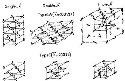
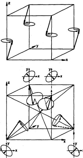
where we have made the assumption that the phases \( \phi_{k} \) can be taken as 0 or \( \pi \) . It is apparent from this that the amplitude observed \( A = |m|/\sqrt{3} \) , but the whole volume of the crystal contributes to each reflection as there are no domains. The intensity is therefore equal to \( (m^{2}/3)xV \) , which is exactly the same as deduced above from the single-k type with an equal domain population. The multi-k structures for the type-I and type-IA magnetic structures are shown in Fig. 2.
Multi-k structures were not new to the actinides – they had been proposed first by Kouvel and Kasper [18] in connection with disordered (Fe,Ni) \( _{3} \) Mn compounds, which also have the FCC crystal structure, but multi-k arrangements are to be found much more frequently in the actinide compounds rather than those of the transition metals. We shall discuss some reasons for this situation. There are two important aspects of the triple-k structure evident from Fig. 2. First, the direction of the moments lies always along a \( \langle111\rangle \) direction, and, second, the overall symmetry of the magnetic structure is cubic. Rossat-Mignod saw immediately that the triple-k structure could answer two of the then current ( \( \sim1976 \) ) puzzles of the UX compounds – why many of the antiferromagnets appeared to remain cubic in the ordered state (Table 1), and why the crystal-field easy axis in USb suggested a \( \langle111\rangle \) direction. Both these 'riddles' coming out of the Argonne measurements were explained by supposing that the magnetic structure was triple-k. Simultaneously, Rossat and his group at CENG started working on the magnetic-phase diagram of the USb-UTe solid solutions; these measurements, together with the magnetization measurements by Vogt and colleagues, gave further credence to the idea that the easy axis throughout this system was \( \langle111\rangle \) [UTc was already known to be an easy \( \langle111\rangle \) ferromagnet, see Table 1] and this made Rossat determined to prove directly that multi-k structures were present.

Fig. 2. Multi-k structures associated with an ordering of type-1 (k = [001]) and type-IA (k = [0,0,0.5]) for the NaCl structure with \( m_{s} \) parallel to k. Only the actinide ions are shown.

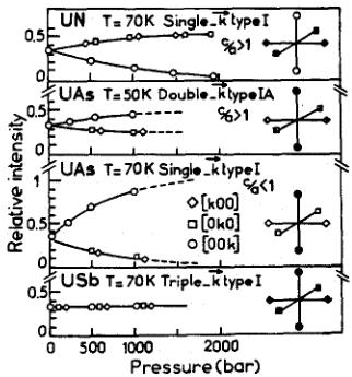
Fig. 3. Effect of uniaxial stress on the relative intensities of the superlattice magnetic peaks associated with the three equivalent wave vectors \( k_{1} = [k00] \) , \( k_{2} = [0k0] \) , and \( k_{3} = [00k] \) for UN, UAs, and USb. The uniaxial stress was applied along the [00l] axis. Only magnetic peaks represented by filled symbols remain after domain re-orientation (taken from Ref. [2]).
4. Experiments to prove the multi-k nature of the structures
The key point in discussing the single and multi-k structures is that the diffracted intensities are the same only when the domain populations have a special value, i.e. \( \frac{1}{3} \) in the case of the triple-k case. The experiments to perform are then to apply an external perturbation sufficiently large to change the domain population in the case of a single-k structure. Ways to do this are to apply a uniaxial stress, cool the material in a large magnetic field (although the choice of which axis to put parallel to the field can often be important), and to examine the material with a surface sensitive probe. We shall give examples of all three.
4.1. Applying uniaxial stress to the UX compounds
It is clear that if the magnetic structure is single-k then the symmetry is tetragonal. The c/a ratio is then likely to be different from unity. If c/a < 1 and a uniaxial stress \( \sigma \) is applied parallel to the [001] direction, then the domains with \( k_{3} = [001] \) will be favored as the stress will reduce the length in the [001] direction at the expense of the other two. In a series of elegant experiments on UN, UAs, and USb, Rossat and his colleagues [19] showed that the application of uniaxial stress of even a small amount led, in certain cases, to the change of the domain population. A summary of the experimental results is shown in Fig. 3. These experiments established

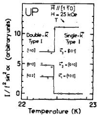
Fig. 4. The dependence of the superlattice magnetic peak intensities in UP as a function of the temperature through the single-k → double-k phase transition in an applied field of 25 kOe (taken from Ref. [2]).
unambiguously that nature of the ordering in UN, UAs, and suggested a triple-k ordering in USb. The difficulty in USb, in which no effect was observed, is that one does not know the threshold stress – however, it appeared almost certain at this stage that USb was, in fact, a triple-k state.
4.2. Cooling in a magnetic field
To obtain similar results with a magnetic field it is necessary to field cool with \( H_{\parallel} \) a two-fold axis, e.g. [1, -1, 0] as shown for the case of UP in Fig. 4 [2]. In the single-k state the \( k_{3} \) domains, which gives rise to the reflection (110), will be favored because \( \chi_{\perp} > \chi_{\parallel} \) , where these directions are with respect to the moment directions of the individual components. For the configuration indicated in Fig. 4, the \( k_{3} \) domain is favored in the single-k structure. In the double-k structure the (xz) and (yz) domains are equivalent, but a slight misorientation of the crystal is enough to favor one over the other. In UAs this method was able even to produce a single domain. It is significant that these experiments on UP, showing a 1k-2k transition at 24 K, resolved a longstanding mystery of why the moment should suddenly 'jump' in value at this temperature. There is a change in direction of the magnetic moments. The increase in the value of the moments comes from them being in the easy direction at the lowest temperature. Earlier theories advanced [20] to 'explain' these effects immediately became suspect with the new understanding from experiments; although, in the case of Robinson and Erdos [20] many of their concepts of hybridization are still recognized as correct.
4.3. Domains as they appear to a surface-sensitive probe
Recently, the use of X-ray resonant magnetic scattering has been applied to actinide compounds \( [21, 22] \) and


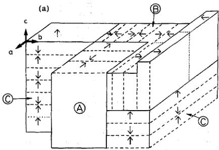
Fig. 5. (a) Schematic drawing of the crystal of NpAs showing the different types of magnetic domains. Each arrow represents 4 magnetic moments (i.e. 2 unit cells). Solid lines represent domain boundaries, dashed lines are changes of moment direction within one domain, and the dotted lines are other possible antiphase domain boundaries. (b) Calculated \( k_{3} \) domain fraction based on the assumption that \( k_{1} \) and \( k_{2} \) domains are equally populated [note that C and \( k_{3} \) domain are equivalent nomenclatures] (taken from Ref. [23]).
the increased wave vector resolution has allowed new details of the magnetic structure to be determined. A good example is the study of NpAs just completed [23]. This technique uses X-rays from a synchrotron tuned to the \( M_{IV} \) absorption edge energy (3.852 keV for Np) and is sensitive to the near-surface volume of the sample because of the high absorption ( \( \mu \) , the linear absorption coefficient \( \sim25\,000\,cm^{-1} \) ) of the photons. The penetration depth of these X-rays is limited to about the first 1200 Å of the material. NpAs orders with a type-I incommensurate structure (see Table 1) and this is known to be a single-k state, because of both the presence of a distortion in this state [10] and experiments in a magnetic field [24]. Fig. 5(a) shows a schematic of the arrangement of the crystal surface with the longitudinal arrangement of single domains indicated. Naturally, there are a number of domain walls, both within a single domain, and between domains. In using neutrons without a magnetic field or uniaxial stress the domain volumes are found to be random, i.e. each domain has a volume of \( \frac{1}{3} \) [25]. The situation is different when using resonant X-rays. A careful experiment is able to establish the fraction of \( k_{3} \) domains (also called C domains) in the volume probed by the X-ray beam, and this is shown in Fig. 5(b). There are a number of interesting regions of Fig. 5(b). First, near \( T_{N} \) there is a slow decrease in the population of the \( k_{3} \) domains; this is because domains with moments pointing out of the surface have a greater dipole energy [26] than those with the moments in the surface plane and the moments rotate to the \( k_{1}(A) \) and \( k_{2}(B) \) domains to minimize the dipole energy. However, in the region between \( T_{N} \) and \( T_{o} \) a tetragonal distortion develops that gradually increases in magnitude on cooling. A glance at Fig. 5(a) shows that this means that inter-domain stresses develop as the c/a ratio steadily decreases from unity. The problem is like trying to pack a series of oblique blocks together. A more favorable configuration is with a single \( k_{3} \) domain in the surface region, the tetragonality can then be easily accommodated without inter-domain stresses. This latter mechanism finally wins out over the dipole energy and a sudden transition to a single-domain \( k_{3} \) state is seen at \( \sim138 \) K. At 130 K. NpAs transforms to a triple-k state, becomes cubic with the easy direction changing from \( \langle001\rangle \) to \( \langle111\rangle \) , becomes a semi-metal, and exhibits a large increase in the volume [10]. What induces this transition is unknown.
Similar X-ray experiments on known triple-k structures, such as USb, \( U_{0.85}Th_{0.15}Sb \) , and USb \( _{0.8}Te_{0.2} \) have not observed these 'domain re-orientation effects' – a further proof of the correctness of our interpretation of these latter structures, as being triple-k in nature.
5. Consequences of the multi-k structures
It was, of course, not simply the determination of the structures that fascinated Jean Rossat-Mignod. He also wanted to think through all their consequences and answer the question why they were formed. We shall discuss first some of the consequences.
5.1. Magnetization measurements on multi-k structures
The production of the UX single crystals in the mid-1970s \( [13] \) (and their extension to the transuranium materials of this structure in the 1980s) allowed detailed magnetization experiments to be performed by Oscar Vogt \( [27] \) and his collaborators in Zürich up to \( \sim100 \) kOe, and to higher fields at the high-field laboratory in Grenoble, France. Since Vogt will be reviewing the

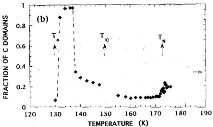
Fig. 6. Magnetic-phasc diagram of UAs as a function of T and H applied along the [00 l] axis. This has been derived from both magnetization ( \( H_{max}=200 \) kOe) and neutron diffraction ( \( H_{max}=100 \) kOe) measurements (taken from Ref. [2]).
mcasurements on CeSb in this volume [28], we will not elaborate on the technique but simply illustrate the results for UAs in Fig. 6. This is a wonderfully complex phase diagram that Rossat took great delight in recalling on numerous occasions. It is vital in the interpretation of the magnetization curves to understand the exact nature of the multi-k structure at any value of T and H. Without such an understanding the magnetization results are incomprehensible.
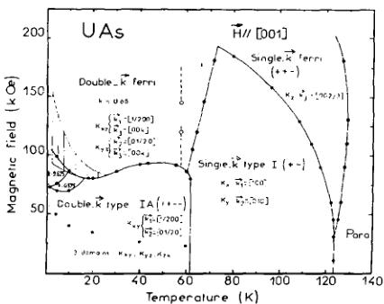
UAs is an exceptionally complex case; it is perhaps more instructive to just examine one aspect of the pseudo-binary compound \( USb_{0.85}Te_{0.15} \) [29]. The magnetization curves are shown in the upper panel of Fig.7. The field here is applied along the [111] axis, which at high fields is the easy axis. The 'jumps' in the magnetization process are associated with the disappearance of the Fourier components of the AF triple-k structure. The k-vector is \( \langle\frac{1}{2}00\rangle \) . At H=20 kOe the \( k_{1} \) component becomes ferromagnetic, leading to an increase of the magnetization, and a decrease to zero of the intensity of the AF peak ( \( \frac{1}{2},1,1 \) ). At higher fields the \( k_{2} \) and \( k_{3} \) components become ferromagnetic. In this particular case it is unclear why these components should change at different fields, as the field H makes the same angle with all three of them. Presumably, strains in the crystal or a slight misorientation will cause the inequality and may not therefore be reproducible from experiment to experiment. On the other hand, one of the clearest signatures of these early measurements on triple-k structures was the finding that, although the easy axis at high field was always \( \langle111\rangle \) , the critical field for inducing a ferromagnetic component was always lower with \( H_{\parallel}\langle100\rangle \) than

Fig. 7. Magnctization (upper) and neutron (lower) data showing the magnetization process in \( U Sb_{0.85} Te_{0.15} \) (taken from Ref. [29]).
with \( H\parallel\langle111\rangle \) . To understand this we note that for \( H\parallel[100] \) the AF components parallel to the field will yield a net magnetization of \( m_{F}=m/\sqrt{3} \) and leaves unchanged the AF components perpendicular to the field. For \( H\parallel[111] \) the field has to flip all three AF components, so that the critical field is higher. However, once the AF components are flipped, the ferromagnetic moment along the body diagonal is greater than along the cube diagonal. This understanding of the magnetization curves led to the realization that the easy axis across the whole USb–UTE solid solution was \( \langle111\rangle \) .
5.2. Neutron inelastic scattering from USb single crystals
In 1977 we obtained enough small single crystals of USb to try the first 3-axis experiment at the Institut Laue Langevin in Grenoble to measure the dynamics of the system [30]. The results were a surprise in that the lowest-energy spin wave was found to be longitudinally polarized, whereas the normal low-energy spin waves are transverse in their polarization. These directions being with respect to the propagation direction of the magnetic structure.
This problem was resolved by Jensen and Bak in 1981 \( ^{[31]} \) with their realization that, from symmetry arguments, the low-energy transverse spin wave in a triple-k structure actually appears as a longitudinal spin-wave with respect to the propagation of the magnetic modulation. The relative motions of the magnetic moments for a spin-wave at the X point, where the motions of the moments in two adjacent (00 l) planes are exactly \( \pi \) out of phase, are shown in Fig. 8. In the so-called L mode the transverse components within each layer cancel out in a pairwise way because the x and y components of the

Fig. 8. Normal spin waves in USb. The wave vector q is parallel to the z axis. Lower diagram: Full lines and vectors belong to the longitudinal mode at the zone center X, whereas the dashed lines correspond to the transverse mode at X. For comparison the transverse spin-wave mode in the single-k structure is shown in the upper frame (taken from Ref. [31]).
magnetic moment are reversed when the translation of \( \left(\frac{1}{2}\right) \) occurs in the triple-k structure. The longitudinal components (z), however, are all in phase. The mode is thus longitudinal and will appear so in a neutron experiment. The second mode, given by the broken vectors, is quite different and is purely transverse – but it is at higher energy. Both these results agreed with the experiments on USb [30] giving direct proof from the neutron inelastic spectrum that the structure of USb is of the triple-k form.
5.3. Questions about the phase angle \(\phi_{k}\) in the triple-k structure
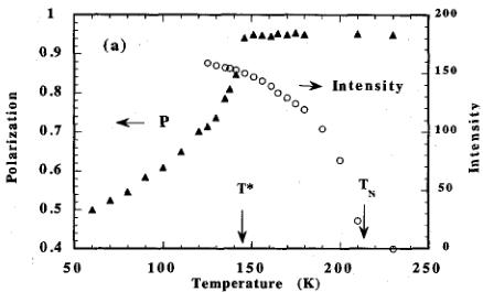
We have seen in Eq. (4) that determining the moment in a triple-k magnetic structure at a given atomic site \( (\pmb{R}_{n}) \) in the chemical structure requires not only the amplitude of the modulation, but also the phase angles \( \phi_{k} \) between the different k components. Diffraction measurements cannot give any information about this phase angle. The diffracted intensities are the same whatever the values of \( \phi_{k} \) . However, the physical picture, such as we have drawn in Fig. 2, depends on these phase angles. If these phase angles change, then a new 'domain' will be produced – although there will be no change in the integrated intensities of the AF Bragg peaks. In particular, as Rossat recognized [19], the gradual changing of \( \phi_{i} \) will result in a soliton-like domain wall propagating through the system. Evidence for such effects is, of course, difficult to establish as we have no physical technique sensitive to the phase angles themselves – only consequences of their behavior. We return to our 'old friend' USb. There have been at least four experiments that have given evidence of some unusual behavior below \( T_{N} \) (= 215 K) in USb. The first is the maximum in the resistivity found at \( \sim \) 145 K by Schoenes et al. [32], the second is the sudden damping of the spin-wave excitations [33] that occurs at \( \sim \) 160 K, the third is the sudden increase of the relaxation rate of the muon spectra [34] that occurs at 150 K, and the fourth is the unusual depolarization effects found recently [35] when a beam of polarized neutrons is passed through USb. Data from the latter study are illustrated in Fig. 9. The depolarization of the neutron beam (E = 14.7 meV) starts abruptly at a temperature \( T^{*} \) which is some 70 K below \( T_{N} \) . No change in the intensity of either the AF or nuclear peaks are observed. What can cause the sudden depolarization of the neutron beam? Bulk ferromagnetism has been ruled out by static magnetization measurements as well as the muon experiments [34]. However, a dynamic ferromagnetic component cannot be excluded by the static measurements. It is simple to show that a changing phase angle \( \phi_{i} \) between certain of the triple-k components can lead to regions of the crystal that have a ferromagnetic component. Because the total bulk moment must be zero, these regions must be balanced by those of oppositely directed moments. However, it is these regions that can cause the change in neutron polarization shown in Fig. 9. Above \( T^{*} \) the regions are either too small, or their dynamics are not matched to the transmittal time of the neutron ( \( \sim \) 1.7 mm/ \( \mu \) s). For example, if the rate of fluctuation becomes large then the neutron will observe a null effect. We can calculate that for a complete Larmor precession of the neutron spin, in which case \( P \rightarrow 0 \) , the spatial extent of this 'domain wall' should be \( \sim \) 50 \( \mu \) m, so that the regions must be considerably smaller than that. Neutron depolarization is a complex process [36], and until this effect is examined as a function of neutron velocity and applied magnetic field no quantitative statements are possible.
We thus have a model that the phase angles vary below \( T^{*} \) and allow microscopic regions (possibly around an


Fig. 9. Depolarization of polarization neutrons as a function of temperature through a single crystal of USb. (a) Variation of the polarization (solid triangles) and the \( (110) \) magnetic intensity (open circles) as a function of temperature. The Néel temperature of this sample is \( 213 \pm 2 \) K. (b) Variation of the Bragg intensities; AF(110)-open circles, and the nuclear(111)-solid squares around the temperature \( T^{*} \) (taken from Ref. [35]).
impurity or at a dislocation in the crystal) to have a ferromagnetic component. As \( T^{*} \) is approached from low temperature the variation of the phase angles increases leading (a) to smaller regions of such a ferromagnetic component and thus a reduction in depolarization, (b) to a poorly defined net moment at each site and thus a damping of the spin waves and strong relaxation of the muon single.
6. Theory of interactions in AnX compounds
6.1. The role of hybridization in defining the planar interactions
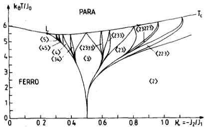
The early work, even on polycrystalline materials, showed that the structures of the AnX derivatives (e.g. in the UP–US solid solutions [5, 6]) could be understood as longitudinal with ferromagnetic (00 1) sheets arranged in a complex manner. Since the only variable in the solid solutions such as UP–US, USb–UTE, and USb–ThSb is the electron concentration (U being almost trivalent in every case), the changing of the structures indicates the importance of interaction with the conduction electrons either through the RKKY or more complex interactions. These ideas were reinforced by the experiments on the critical scattering of first USb [37], then many other AnX materials, including UAs [38], PuSb [39], and also the CeX compounds [40]. These showed unambiguously that the interactions within a ferromagnetic (00 1) plane were much stronger than the interactions between the planes. We should emphasize that these statements apply to each component of the multi-k structure – see Ref. [38] for a complete discussion of this point. This anisotropy has led to at least two important developments: (1) It allows discussions of the interactions to introduce anisotropic interactions between the uranium 5f wave functions and either (or both) the conduction electron states [41] or the anion p states [42]. The former appears the more important in the case of the actinide systems with 5f electrons, whereas the latter may be more applicable to the case of cerium compounds with 4f electrons. The oblate wave functions surround the uranium site, and hybridizing primarily in the ferromagnetic (00 1) plane as shown in Fig. 1, is an example of the mechanism proposed by Ref. [42]. Cooper and his colleagues have gone on to examine the consequences of anisotropic hybridization with the band states in the dynamic behavior [43] of the AnX materials, and the agreement with experiment obtained shows a postiori the importance of this hybridization mechanism. Having developed a microscopic mechanism to couple the moments in (00 1) ferromagnetic sheets, with a weak coupling between the sheets, we can turn to (2) the second class of theories that treats the consequences of such an interaction and the subsequent phase transitions. The problem may be reduced to a one-dimensional problem involving the ordering wave vector k, which just has a component along the one dimension, say \( k_{3} \) . Group theoretical models developed by Bak and von Boehm [44], Selke and Fisher [45], Villain and Gordon [46], and others have shown that the problem reduces to the so-called ANNNI model, in which a vast number of commensurate phases may be stabilized, in the end reducing to a devil's staircase in which almost all fractions n/m, where these are integers, may be found. The exchange interaction within the (00 1) sheets is the strongest and is labeled \( J_{0} \) , whereas exchange interactions between the planes being \( J_{1} \) for the nearest neighbor, and \( J_{2} \) for the next-nearest neighbor. Since the (00 1) planes are ferromagnetically aligned \( J_{0} > 0 \) , the phase diagram may be mapped for values of \( J_{2}/J_{1} \) . An example, taken from Ref. [47] is given in Fig. 10.
These theories give a great deal of information about the phase diagrams but they are complementary to the theories discussed earlier as they do not depend on

Fig. 10. Mean field diagram of the simple ANNNI model, showing the main commensurate phase. This corresponds to the case of the AnX compounds in which \( J_{0} > 0 \) . Here a structure such as \( \langle 4 \rangle \) means an arrangement 4 -, 5 +, 4 +, 5 -, as found, for example, in the UP-US solid solution [6]. L marks a Lifshitz point instability. It has been proposed that UAs is near such a point [38] (taken from Ref. [47]).
the microscopic origin of the interactions, only their symmetry. The combination of these two types of theories allows many of the complications of the AnX phase diagrams to be understood including many subtle effects relating to the incommensurate to commensurate phase transitions, but they do not tell us why multi-k structures develop.
6.2. Reasons for the multi-k structures
If we take a single Bravais lattice (corresponding, for example, to the triple-k structure of USb) then we can write the free energy of the system in Fourier space [16]:
\[ \begin{aligned}f_{(\mathbf{k})}=&f_{0}+a_{\mathbf{k}}\sum_{i}m_{\mathbf{k}i}m_{-i}+b_{\mathbf{k}}\sum_{i}m_{\mathbf{k}i}^{4}+b_{\mathbf{k}}^{\prime}\sum_{i\neq j}m_{\mathbf{k}i}^{2}m_{\mathbf{k}j}^{2}\\&+c_{\mathbf{k}}\sum_{i}m_{\mathbf{k}i}^{6}+c_{\mathbf{k}}^{\prime}\sum_{i>j}m_{\mathbf{k}i}^{4}m_{\mathbf{k}j}^{2}+c_{\mathbf{k}}^{\prime\prime}\sum_{i\neq j,i}m_{\mathbf{k}i}^{2}m_{\mathbf{k}j}^{2}m_{\mathbf{k}i}^{2},\end{aligned} \quad (5) \]
where this represents the case with \( m_{k} \parallel k \) and the summation is made over the wave vectors \( k_{i} \) of the star \( \{k\} \) . In our case this contains three members, \( k_{1} = [100] \) , \( k_{2} = [010] \) , and \( k_{3} = [001] \) . This equation shows that up to second order the free energy does not contain any terms that come from a coupling between the different k vectors. To remove the degeneracy between the single- and multi-k structures we have to introduce terms in at least the fourth-order. If only fourth-order terms are taken into account then the structure will be single or triple-k depending whether \( b_{k}^{\prime} \) is negative (triple-k) or positive (single-k). The addition of the sixth-order terms allows the possibility that a double-k structure may be stabilized. This, of course, is consistent in that to produce a \( \langle 1\ 10\rangle \) (2-fold) easy axis in a cubic system the crystal-field potential should contain large sixth-order terms.

Fig. 11. Possible triple-k structures associated with the wave vector \( \langle\frac{1}{2}\frac{1}{2}0\rangle \) and a simple cubic lattice (taken from Ref. [49]).
The stabilization of the multi-k structures requires the presence of these high-order terms in the free energy, but does not, of course, tell us where they come from. With purely Heisenberg interactions and only single-ion anisotropy the single-k structure is favored. The presence of a large anisotropic hybridization in the actinides leads in a straightforward way to the presence of such higher-order terms in the free energy.
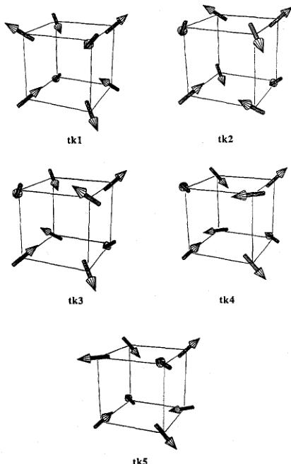
The difficulty is not in identifying the type of interactions that must be responsible for the multi-k structures in the AnX compounds, but in establishing a quantitative description. Take, for example, the case of the lanthanide compounds, many of which have complicated structures as well. The advantage in most cases is that here many of the interactions are known extremely well, and measurements such as magnetostriction and elastic constants can be made which isolate various contributions to the free energy \( [48] \) . In particular, quadrupolar interactions play an important part in stabilizing the multi-k structures found in lanthanide compounds. We show in Fig. 11 all
the possible 3k structures deduced [49] with a wave vector \( \left\langle\frac{1}{2}\right\rangle \) . This wave vector is not actually found in the AnX compounds, but applies to the case of the compound \( NdIn_{3} \) [49], in which the Nd ions are on a simple cube. The interactions, primarily quadrupolar, that lead to this kind of magnetic ordering can be defined precisely, and their temperature dependence often leads to transitions from one structure to another. All the higher-order interactions such as crystal-field and quadrupolar are well known. What is interesting is seeing whether the phase transitions as a function of H and T can be understood in a consistent fashion.
A similar attempt in the AnX compounds immediately encounters the difficulty of defining the crystal–field interaction. This remains one of the central problems in these materials – it is now known that the hybridization essentially ‘washes out’ the crystal–field excitations, so that in the technique of neutron inelastic scattering they cannot be observed \( [50, 51] \) . Quadrupolar effects are certainly important as well, but the high ordering temperatures and large direct exchange interactions, as well as the anisotropy of these exchange interactions, makes them difficult to isolate. In another actinide compound, \( UO_{2} \) , the \( T_{N}(30\ K) \) is low enough so that the quadrupolar 3k nature of the phase transition \( [52] \) could be established by investigating the H–T phase diagram \( [53] \) . Quadrupolar effects were predicted \( [54] \) to be responsible for the phase transition in UAs at \( T_{N}/2 \) , but the recent observation \( [21] \) of the small internal arrangement of the anion sublattice suggests these effects are a consequence rather than a cause for the \( 1k \rightarrow 2k \) transition (at \( T_{N}/2 \) ) in UAs.
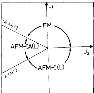
Monachesi and Weling [55] essentially took the Hamiltonian giving rise to Eq. (5) and considered the case of the AnX compounds. They took the crystal-field parameters from the form-factor work [15] on USb, and showed that the magnetic phases could be deduced. The relative values of the exchange parameters \( J_{0} > J_{1} \) and \( J_{2} \) are shown in Fig. 12. The crystal-field interaction in this theory is crucial in determining whether a multi-k structure exists; in practice other higher-order interactions, such as quadrupolar effects, may also be important.
7. Recent developments in the AnX compounds
Work continues in a number of directions in this field. The new technique of resonant X-ray scattering \( [21, 22] \) has been applied to UAs \( [21] \) , \( U_{0.85}Th_{0.15}Sb \) \( [56] \) , \( USb_{0.8}Tc_{0.2} \) \( [57] \) , and more recently to USb \( [58] \) itself. The advantage of this technique is the higher wave vector resolution available than with conventional neutron diffraction. In the case of NpAs \( [23] \) we have already discussed one aspect of the measurements (scc f·ig. 5), and

Fig. 12. Magnetic phase of U pnictides in terms of the \( J_{1} \) parameters defined in the text. \( J_{0} > 0 \) and greater than the other interactions. The \( Al^{+} \) type-IA and type-I phases corresponding to UN, UP, and USb are stable (taken from Ref. [55]).
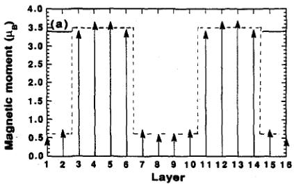
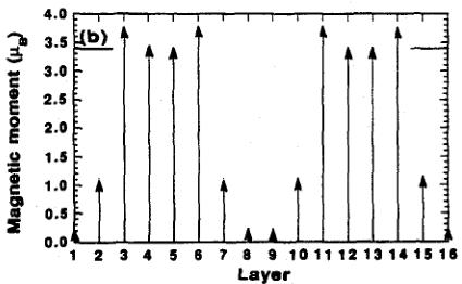
the measurements [23] in the incommensurate state have been able to show evidence for the 'devil's staircase' behavior discussed earlier [44–47]. The study on \( U_{0.85}Th_{0.15}Sb \) [56] addressed another question that has been present since the early days of research on solid solutions. When more than one component is present in the diffraction pattern can we be sure that they come from the same microscopic volume of the crystal? Or, put another way, are the crystals multiphase? In some cases, of course, the answer to the latter is clearly yes, but, in the case of \( U_{0.85}Th_{0.15}Sb \) the authors argued on the basis of the sharpness of the charge peaks that all four magnetic components existed in the same volume of the crystal. Recalling the difficulty in combining components in the absence of information of the phase, the authors proposed a number of different modulations for the structure, and these are shown in Fig. 13. The magnitudes of the moments in Fig. 13 were obtained by minimizing the entropy (i.e. attempting to minimize the difference between the magnitudes of adjacent moments) and represents only one series of possible models. Since the \( \langle111\rangle \) direction is the easy axis and a ferromagnetic component exists in this direction, it is difficult to imagine the precise directions of the moments at each site, remembering that the other components are all of the 3k form. However, we may still consider the magnitude of the moment as a defined quantity. The interesting aspect is that this modeling produces almost paramagnetic planes in the ordered state. These have not been found previously in AnX materials, but are a common feature of the phase diagrams of CeX compounds [59 61], and were once of the major discoveries of Rossat and his colleagues in their early studies of CeSb [59].


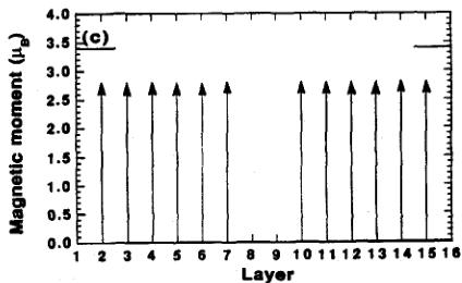
Fig. 13. Models of the magnetic configuration at low temperature in \( U_{0.85}Th_{0.15}Sb \) . The horizontal line at \( 3.4\mu_{B} \) is the maximum moment in the \( 5f^{3} \) state. In each case two repeat units (4 unit cells) are shown. The modulation is longitudinal, but is shown transverse for convenience. (a) Results of adding components \( k=0, k=0.25 \) and \( k=0.75 \) . The square-wave modulation is shown as a broken line. (b) Adding the k=0.5 component. (c) The \( 6+ \) , 0, 0 structure suggested by the X-ray intensities in the low-temperature state (taken from Ref. [56]).
In the same study of \( U_{0.85}Th_{0.15}Sb \) [56] the authors also noted that all magnetic peaks were considerably wider than the experimental resolution despite the magnetic structure being commensurate. Maximum coherence lengths of \( \xi\sim300\AA \) were found illustrating the number of 'faults' present in such a complex magnetic
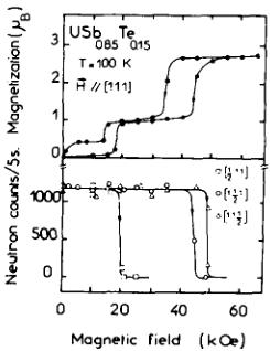
(a)

(b)

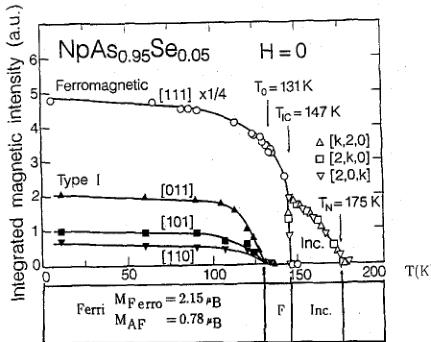
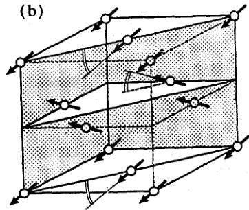
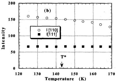
Fig. 14. (a) Intensities of various magnetic peaks in the compound \( NpAs_{0.95}Se_{0.05} \) as a function of temperature. (b) Noncollinear ferrimagnetic structure of the material (taken from Ref. [65]).
arrangement. Presumably 'faults' are needed to relieve the magnetoelastic strain in such an arrangement as shown in Fig. 13. Interestingly, a limited coherence length was also found in the ordered AF state of the heavy fermion material \( URu_{2}Si_{2} \) by resonant X-ray scattering [62], although with a very small moment of \( \sim0.04\mu_{B} \) magnetoelastic effects are likely to be small and another explanation is required.
As indicated by Table 1, the details of the magnetic structures of the Np and Pu monopnictides are now also known from experiments on single crystals \( [63, 64] \) , and we find similar features in the magnetic structures – indeed NpAs has a phase diagram of at least equal complexity to that found in UAs. Solid solutions of some of these compounds are now being investigated and we show in Fig. 14 the results from a study \( [65] \) of the solid solution.
between NpAs and NpSe. Neither of these pure compounds has a ferromagnetic component (Table 1), but when a small amount of Se is doped into NpAs a ferromagnetic component develops, and the easy axis is found to be \( \langle110\rangle \) . The resulting noncollinear magnetic structure is shown in Fig. 14(b). This is the first time a real noncollinear structure has been established, and it comes (surprisingly) in a system in which both the triple-k structure in NpAs and the NpSc magnetic structure have \( \langle111\rangle \) as the easy axis. That this occurs at such a small electron doping (only 5% NpSe) is consistent with the work on UX UZ (X = pnictide, Z = chalcogenide) systems in which the value of the k-vector systems change rapidly with small changes in the electron concentration.
8. Conclusions
The complex magnetic structures of the AnX compounds are a direct consequence of many of the characteristics (e.g. hybridization) that make the research on actinide compounds so fascinating. Nobody saw this more clearly than Jean Rossat-Mignod. His long experience in the magnetic properties associated with lanthanide compounds, his tenacity when a problem was 'unsolved', his ability to enlist the help and infect others with his enthusiasm, and his profound knowledge of physics, were all put to perhaps their greatest use in his unrelenting efforts over a period of \( \sim \) 15 years to 'understand' these materials. Enormous progress has been made, much of it attributable to Rossat and his collaborators at Grenoble. More remains to be done.
We have already indicated many of the puzzles remaining. Perhaps the most outstanding problem is to try to understand the dynamic properties of these materials. A number of neutron inelastic experiments have been performed \( [30, 40, 50, 51] \) , but very little is known about the transuranium materials. Since we expect increased localization as we progress across the actinide series, it may be easier to understand (but certainly not easier to measure!) the excitations of Pu as compared to U compounds, and the one experiment on PuSb \( [66] \) bears this out, although the results are not so straightforward to interpret \( [67] \) . Rossat was a great advocate of these kinds of measurements to allow a more detailed understanding of the microscopic interactions involved. He pushed unrelenting for larger crystals from Zürich and Karlsruhe! A profitable area would seem also to be the field of dilution with materials such as La or Y. A start of doping both US and UTe with such nonmagnetic species has begun \( [27, 68] \) , and the results (predictably!) are interesting. Rossat spent a considerable effort trying to encourage de Haas–van Alphen measurements on these materials, but it seems that (at least up to now) the quality of the crystals has not been good enough or the electron orbits not long enough. Real details about the Fermi surface would be of great value.
The Mössbauer technique is particularly appropriate for the Np nucleus \( [69] \) and has added much to our knowledge of the NpX compounds. The technique has also been used to measure the magnetic properties up to about 10 GPa (100 kbar) and is thus complementary to the technique of the measurement of resistivity as a function of T with the pressure varying up to \( \sim25 \) GPa \( [70] \) . The measurement of the L-edge absorption spectra as a function of pressure is another promising technique to investigate the electronic structure \( [71] \) . The systematics of the phase transitions under pressure are as yet unclear, and it is particularly frustrating that microscopic probes, such as neutron diffraction, can only with great difficulty arrive at \( \sim10 \) GPa. Again it was Rossat who was the driving force behind some of these developments in high-pressure diffraction, and it is significant that the first results were obtained on UAs \( [72] \) . This was completely in character for him, just as 10 years before he had demanded (and got!) a 100 kOe magnet at the CEN-Grenoble \( [19] \) .
Note added in proof: Some de Haas–van Alphen experiments on USb have recently been reported [73].
Acknowledgements
We owe, of course, a special debt to Jean Rossat-Mignod as this paper makes abundantly clear. He gave many of us 'orders' and they were usually right – many of us knew him simply as the 'chief'! We thank especially Oscar Vogt, Kurt Mattenberger and Barry Cooper for 20 years of cnjoyable collaboration. Many others, always inspired by Rossat's enthusiasm, played major roles. Moshe Kuznietz started much of it but joined with Rossat in France. Jean-Pierre Sanchez, Bill Stirling, and Simone Quezel were part of 'his' team in Grenoble, and Jean-Claude Spiret and Jean Rebizant were in Karlsruhe. Paul Burlcet is also supported by the CNRS.
References
[1] C.G. Shull and J.S. Smart, Phys. Rev. 76 (1949) 1256.
[2] J. Rossat-Mignod, G.H. Lander and P. Burlet, in: Handbook on the Physics and Chemistry of the Actinides, Vol. 1, eds. A.J. Freeman and G.H. Lander, (North-Holland, Amsterdam, 1984) p. 415 and references therein.
[3] G.H. Landcr, M. Kuznietz and Y. Baskin, Solid State Commun. 6 (1968) 877.
[4] J.S. Smart, Effective Field Theories of Magnetism (Saunders, Philadelphia, 1966).
[5] M. Kuznietz, G.H. Lander and Y. Baskin, J. Appl. Phys. 40 (1969) 1130.
[6] G.H. Lander, M. Kuznietz and D.E. Cox, Phys. Rev. 188 (1969) 963.
[7] J. Leciejewicz, A. Murasik, R. Troc and T. Palewski, Phys. Stat. Sol. 46 (1971) 391.
[8] G.H. Lander, M.H. Mueller and J.F. Reddy, Phys. Rev. B 6 (1972) 1880.
[9] J. Grunzweig-Genossar, M. Kuznietz and F. Friedman, Phys. Rev. 173 (1968) 562.
[10] A.T. Aldred, B.D. Dunlap, A.R. Harvey, D.J. Lam, G.H. Lander and M.H. Mueller, Phys. Rev. B 9 (1974) 3766.
[11] W.L. McMillan, Phys. Rev. B 14 (1976) 1496.
[12] G.H. Lander and M.H. Mueller, Phys. Rev. B 10 (1974) 1994.
[13] J.C. Spirlet and O. Vogt, in: Handbook on the Physics and Chemistry of the Actinides, Vol. 1, eds. A.J. Freeman and G.H. Lander (North-Holland, Amsterdam, 1984) p 79.
[14] N.A. Curry, Proc. Phys. Soc. (London) 86 (1965) 1193.
[15] G.H. Lander, M.H. Mueller, D.M. Sparlin and O. Vogt, Phys. Rev. B 14 (1976) 5035.
[16] J. Rossat-Mignod, in: Neutron Scattering, eds. K. Skold and D.L. Price, Methods of Experimental Physics, Vol. 23C (Academic Press, New York, 1987) p. 69.
[17] G.H. Lander, in: Handbook on the Physics and Chemistry of Rare Earths, Vol. 17 eds. K.A. Gschneidner, L. Eyring, G.H. Lander and G. Choppin (Elsevier, Amsterdam, 1993) p. 635.
[18] J.S. Kouvel and J.S. Kasper, J. Phys. Chem. Solids 24 (1963) 529.
[19] J. Rossat-Mignod, P. Burlet, S. Quezel and O. Vogt, Physica B 102 (1980) 237.
[20] J.M. Robinson and P. Erdos, Phys. Rev. B 8 (1973) 4333; Phys. Rev. B 9 (1974) 2187.
[21] D.B. McWhan, C. Vettier, E.D. Isaacs, G.E. Ice, D.P. Siddons, J.B. Hastings, C. Peters and O. Vogt, Phys. Rev. B 42 (1990) 6007.
[22] G.H. Lander and W.G. Stirling, Physica Scripta T45 (1992) 15.
[23] S. Langridge, W.G. Stirling, G.H. Lander and J. Rebizant, Phys. Rev. B 49 (1994) 12 010; Phys. Rev. B 49 (1994) 12 022.
[24] P. Burlet, D. Bonnisseau, S. Quezel, J. Rossat-Mignod, J.C. Spirlet, J. Rebizant and O. Vogt, J. Magn. Magn. Mater. 63-64 (1987) 151.
[25] D.L. Jones, W.G. Stirling, G.H. Lander, J. Rebizant, J.C. Spirlet, M. Alba and O. Vogt, J. Phys. CM 3 (1991) 3551.
[26] J.G. Gay and R. Richter, Phys. Rev. Lett. 56 (1986) 2728.
[27] O. Vogt and K. Mattenberger, in: Handbook on the Physics and Chemistry of Rare Earths, Vol. 17, eds. K.A. Gschneidner, L. Eyring, G.H. Lander and G. Choppin (Elsevier, Amsterdam, 1993) p. 301.
[28] O. Vogt, Physica B 215 (1995) 22.
[29] J. Rossat-Mignod, P. Burlet, S. Quezel, O. Vogt and H. Bartholin, in: Crystalline Electric Fields in f-electron Magnetism, eds. R. Guertin, W. Suski and Z. Zolnierek, (Plenum, New York, 1982) p. 501.
[30] G.H. Lander, W.G. Stirling and O. Vogt, Phys. Rev. Lett. 42 (1979) 260; Phys. Rev. B 21 (1980) 436.
[31] J. Jensen and P. Bak, Phys. Rev. B 23 (1981) 6180.
[32] J. Schoenes, B. Frick and O. Vogt, Phys. Rev. B 30 (1984) 6578.
[33] M. Hagen, W.G. Stirling and G.H. Lander, Phys. Rev. B 37 (1988) 1846.
[34] L. Asch, G.M. Kalvius, A. Kratzer, F.J. Litterst, F.N. Gygax, A. Schenk, K. Mattenberger and O. Vogt, Hyperfine Interactions 64 (1990) 453.
[35] G.H. Lander and S.M. Shapiro, Physica B 213 & 214 (1995) 125.
[36] S. Mitsuda and Y. Endoh, J. Phys. Soc. Japan 54 (1985) 1570; Y. Endoh, S. Itoh, T. Watanabe and S. Mitsuda, Physica B 180–181 (1992) 34.
[37] G.H. Lander, S.K. Sinha, D.M. Sparlin, and O. Vogt, Phys. Rev. Lett. 40 (1978) 523.
[38] S.K. Sinha, G.H. Lander, S.M. Shapiro and O. Vogt, Phys. Rev. B 23 (1981) 4556.
[39] P. Burlet, J. Rossat-Mignod, G.H. Lander, J.C. Spirlet, J. Rebizant and O. Vogt, Phys. Rev. B 36 (1987) 5306.
[40] B. Halg and A. Furrer, J. Appl. Phys. 55 (1984) 1860; Phys. Rev. B 34 (1986) 6258.
[41] B.R. Cooper, R. Siemann, D. Yang, P. Thayamballi and A. Banerjea, in: Handbook on the Physics and Chemistry of the Actinides, Vol. 2, eds. A.J. Freeman and G.H. Lander (North-Holland, Amsterdam 1985) p. 435 and references therein; N. Kioussis and B.R. Cooper, Phys. Rev. B 34 (1986) 3261.
[42] K. Takegahara, H. Takahashi, A. Yanasa and T. Kasuya, Solid State Commun. 39 (1981) 857; J. Phys. C 18 (1985) 2695.
[43] G.J. Hu and B.R. Cooper, Phys. Rev. 48 (1993) 12743.
[44] P. Bak and J. von Boehm, Phys. Rev. B 21 (1980) 5291; note that a paper discussing these effects particularly with respect to CeSb is also by the same authors, Phys. Rev. Lett. 42 (1979) 122.
[45] W. Selke and M.E. Fisher, Phys. Rev. B 20 (1979) 257; Phys. Rev. Lett. 44 (1980) 1502.
[46] J. Villain and M. Gordon, J. Phys. C 13 (1980) 3117.
[47] W. Selke and P.M. Duxbery, Z. Phys. B 57 (1984) 49.
[48] P. Morin and D. Schmitt, in: Ferromagnetic Materials, Vol. 5, ed. K.H.J. Buschow (Elsevier Science, Amsterdam, 1990) p. 1.
[49] M. Amara, Thesis presented to the University Joseph Fourier, Grenoble, 1994 (unpublished); Physica B 210 (1995) 157.
[50] W.J.L. Buyers and T.M. Holden in: Handbook on the Physics and Chemistry of the Actinides, Vol. 2, eds A.J. Freeman and G.H. Lander (North-Holland, Amsterdam, 1985) p. 239.
[51] E. Holland-Moritz and G.H. Lander, in: Handbook on the Physics and Chemistry of Rare Earths, vol. 19, eds. K.A. Gschneidner, L. Eyring, G.H.Lander and G. Choppin (Elsevier, Amsterdam, 1994) p. 1–121.
[52] J. Faber and G.H. Lander, Phys. Rev. B 14 (1976) 1151.
[53] P. Burlet, J. Rossat-Mignod, S. Quezel, O. Vogt, J.C. Spirlet and J. Rebizant, J. Less-Common Met. 121 (1986) 121.
[54] B.R. Cooper, Phys. Rev. B 17 (1978) 293.
[55] P. Monachesi and F. Weling, Phys. Rev. B 28 (1983) 270.
[56] J.A. Paixão, G.H. Lander, C.C. Tang, W.G. Stirling, A. Blaise, P. Burlet, P.J. Brown and O. Vogt, Phys. Rev. B 47 (1993) 8634.
[57] W.J. Nuttall, S. Langridge, W.G. Stirling, G.H. Lander, B. Lebech and D. Gibbs, Phys. Rev. B, in press.
[58] S. Perry, W.J. Nuttall, W.G. Stirling, G.H. Lander and D. Gibbs (unpublished).
[59] J. Rossat-Mignod, P. Burlet, H. Bartholin, J. Villain, W.T. Si, D. Florence and O. Vogt, Phys. Rev. B 16 (1977) 440.
[60] J. Villain, M.B. Gordon and J. Rossat-Mignod, Physica B 102 (1980) 262.
[61] J. Rossat-Mignod, M. Effantin, P. Burlet, T. Chattodpadyhay, L.P. Regnault, H. Bartholin, C. Vettier, O. Vogt, D. Ravot and J.C. Achart, J. Magn. Magn. Mater. 52 (1985) 111.
[62] E.D. Isaacs, D.B. McWhan, R.N. Kleinman, D.J. Bishop, G.E. Ice, P. Zscak, B.D. Gaulin, T.E. Mason, J.D. Garrett and W.J.L. Buyers, Phys. Rev. Lett. 65 (1990) 3185.
[63] P. Burlet, J. Fournier, E. Pleska, S. Quezel, J. Rossat-Mignod, J.C. Spirlet, J. Rebizant and O. Vogt, J. Phys. (Paris) 49 (1988) C8-469.
[64] P. Burlet, F. Bourdarot, J. Rossat-Mignod, J.P. Sanchez, J.C. Spirlet, J. Rebizant and O. Vogt, Physica B 180–181 (1992) 131.
[65] K. Mattenberger, O. Vogt, J. Rebizant, J.C. Spirlet, F. Bourdarot, P. Burlet, J. Rossat-Mignod, M.N. Bouillet and J.P. Sanchez, J. Magn. Magn. Mater. 104 107 (1992) 43.
[66] G.H. Lander, W.G. Stirling, J. Rossat-Mignod, J.C. Spirlet, J. Rebiziant and O. Vogt, Physica B 136 (1986) 409.
[67] A. Banerjea and B.R. Cooper, Phys. Rev B 34 (1986) 1607.
[68] K. Mattenberger and O. Vogt, Phys. Scripta T45 (1992) 103.
[69] W. Potzel, G.M. Kalvius and J. Gal in: Handbook on the Physics and Chemistry of Rare Earths, Vol. 17, eds. K.A. Gschncidner, L. Eyring, G.H. Lander and G. Choppin (Elsevier, Amsterdam, 1993) p. 539.
[70] P. Link, U. Benedict, J. Wittig and H. Wühl. J. Phys. CM 4 (1992) 5585; M. Amanowicz, D. Braithwaite, V. Icbas, U. Benedict, J. Rebizant and J.C. Spirlet, Phys. Rev. B 50 (1994) 6577.
[71] G. Kalkowski, G. Kaindl, S. Bertram, G. Schmiester, J. Rebizant, J.C. Spirlet and O. Vogt, Solid State Commum. 64 (1987) 193.
[72] I.N. Gontcharenko, J.-M. Mignot, J. Rossat-Mignod, V.A. Somenkov and I.V. Naoumov, Physica B 199&200 (1994) 625.
[73] A. Ochiai, F. Hotta, Y. Haga, T. Suzuki, Y. Suzuki, T. Shikama and K. Suzuki, Physica B 206&207 (1995) 789.
 p10_0.jpg
 p10_1.jpg
 p11_0.jpg
 p12_0.jpg
 p12_1.jpg
 p12_2.jpg
 p12_3.jpg
 p12_4.jpg
 p2_0.jpg
 p4_0.jpg
 p5_0.jpg
 p5_1.jpg
 p6_0.jpg
 p6_1.jpg
 p7_0.jpg
 p7_1.jpg
 p8_0.jpg
 p9_0.jpg
 p9_1.jpg