| Transition Temperature | 18 K |
|---|---|
| Experiment Temperature | 4.2 K |
| Propagation Vector | k1 (0, 0, 0) |
| Parent Space Group | R-3c (#167) |
| Magnetic Space Group | C2/c (#15.85) |
| Magnetic Point Group | 2/m (5.1.12) |
| Lattice Parameters | 4.66180 4.66180 14.96300 90.00 90.00 120.00 |
|---|---|
| DOI | 10.1088/0022-3719/6/8/008 |
| Reference | P.J. Brown, P.J. Welford and J.B. Forsyth, Journal of Physics C: Solid State Physics (1973) 6 1405-1421. |
| Label | Element | Mx | My | Mz | |M| |
|---|---|---|---|---|---|
| Co1 | Co | 1. | 2. | 0.0 | 1.73 |
Magnetization density and the magnetic structure of cobalt carbonate
To cite this article: P J Brown et al 1973 J. Phys. C: Solid State Phys. 6 1405
View the article online for updates and enhancements.
Related content
-
A neutron diffraction study of weak ferromagnetism in nickel fluoride P J Brown and J B Forsyth
-
The spatial distribution of ferromagnetic moment in \( MnCO_{3} \) P J Brown and J B Forsyth
-
A search for spin-orbit coupling effects in magnetic neutron scattering by \( FeCO_{3} \) P J Brown and J B Forsyth
Recent citations
-
MAGNDATA: towards a database of magnetic structures. I. The commensurate case Samuel V. Gallego et al
-
Uniaxial magnetic anisotropy of rhombohedral CoCO₃ crystals at T = 0 K V. V. Men'shikov et al
-
Observation of a spin wave exponent of 5/2 in the uniaxial antiferromagnet MnF2SUB22/SUB> Kö et al
Magnetization density and the magnetic structure of cobalt carbonate
P J Brown†, P J Welford† and J B Forsyth‡
†Cavendish Laboratory, Cambridge
‡Neutron Beam Research Unit, SRC Rutherford Laboratory, Chilton, Berkshire
Received 8 November 1972
Abstract. Single crystal diffraction measurements using both polarized and unpolarized neutrons have been made on \( CoCO_{3} \) at 4·2 K. The measurements of the antiferromagnetic reflections have been used to establish a magnetic structure in which the cobalt moments lie wholly within the basal plane. This conclusion, which is contrary to that of previous workers, is a consequence of making a proper calculation of both spin and orbital scattering by the cobalt ion. This calculation is based on a model ground state wavefunction for the cobalt ion in the structure of the carbonate deduced from spectroscopic and magnetization data. The model has also been used in calculating the scattering to be expected from the weak ferromagnetic component of moment which has been measured using the polarized neutron technique. The small differences between the observed scattering and that calculated for the model can in all cases be understood from the difference density distributions as being a consequence of covalency.
1. Introduction
Until recently, detailed studies of magnetization distribution in solids have been confined to materials in which there is little or no orbital moment. In particular, no such studies have been made of ionic materials containing \( Co^{2+} \) . The magnetic neutron scattering cross-section arises jointly from spin and orbital angular momentum. It is well known that the Fourier transform of the spin density can be obtained directly from the amplitudes of the spin scattering, but no such simple relationship exists for orbital scattering. Orbital scattering is also important in many rare-earth ions and Steinsvoll et al (1967) have shown that in general the Fourier transform of the magnetic scattering amplitude gives the magnetization density and in particular have shown how to calculate the spin and orbital contributions to this density. They apply their method to the analysis of their observations of the magnetic scattering from terbium. In this paper we exploit the same method in the first detailed analysis of scattering by \( Co^{2+} \) ions.
Certain rhombohedral, antiferromagnetic crystals such as \( CoCO_{3} \) , \( MnCO_{3} \) and \( \alpha-Fe_{2}O_{3} \) exhibit a spontaneous weak magnetization which arises because the angle between the moments on the two magnetic sublattices is not exactly \( 180^{\circ} \) . Moriya (1960) has developed the theory of an anisotropic superexchange interaction proposed by Anderson (1959) to explain the origin of such weak ferromagnetism. In this theory the ferromagnetism is a direct consequence of intra-atomic spin-orbit coupling linked to the crystal structure. \( Mn^{2+} \) and \( Fe^{3+} \) are S state ions so that the ground state has to a
first approximation no orbital moment. Their very small ferromagnetic moments arise from perturbations of the pure S state by spin-orbit coupling. This has been treated in detail for \( \alpha \) -Fe \( _{2} \) O \( _{3} \) by Kaplan (1964). The ferromagnetism is very much larger in CoCO \( _{3} \) because of the orbital moment of the Co \( ^{2+} \) ion.
2. Previous work
The magnetic properties of \( CoCO_{3} \) were first investigated by Borovik-Romanov and Orlova (1957). Below the critical temperature of \( 18\cdot1~K~CoCO_{3} \) becomes an antiferromagnet in which the moments of the two sublattices do not fully compensate each other. From the results of a powder neutron diffraction experiment Alikhanov (1961) concluded that the spins are inclined at an angle of \( 46^{\circ}\pm4^{\circ} \) to the trigonal axis. This result was, however, deduced from a measurement of only two magnetic reflections and without a reliable form factor for the cobalt ion.
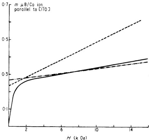
Weak ferromagnetism in a single crystal of cobalt carbonate was investigated by Borovik-Romanov and Özhogin (1961) and the spontaneous ferromagnetic moment extrapolated to 0 K was found to be \( 0.258 \mu_{B} mol^{-1} \) . Their measurements of the moment induced at 4·2 K by fields applied in the basal plane are indicated by the solid curve in figure 1. The thermodynamic theory of weak ferromagnetism given by Dzyaloshinskii

Figure 1. Magnetization of \( CoCO_{3} \) . The full curve is deduced from the measurements of Borovik-Romanov and Özhogin (1961). The other two lines indicate the magnetization predicted by the two forms of the exchange energy described in the text.
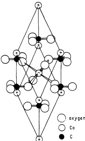
(1957) shows that in crystals with the symmetry of \( CoCO_{3} \) the ferromagnetic moment should lie at right angles to the trigonal axis. \( CoCO_{3} \) has a rhombohedral unit cell \( a_{0}=5\cdot6651\pm0\cdot0001\mathring{A} \) , \( \alpha=48^{\circ}33'\pm3' \) , space group \( R\bar{3}c \) and the \( NaNO_{3} \) type structure illustrated in figure 2. This description of the unit cell rather than the alternative hexagonal one will be used throughout this paper. Below the Néel temperature the

Figure 2. The structure of cobalt carbonate.
spins on alternate cobalt atoms along the trigonal axis have an ordered array such that the moments are not quite antiparallel. The weak ferromagnetic component of the moment is in the plane at right angles to the trigonal axis.
3. Experimental
3.1. X ray structure refinement
No determination appears to have been made of the positional parameter of the oxygen atom in \( CoCO_{3} \) . For this reason an x ray structure refinement was carried out on a small single crystal of \( CoCO_{3} \) . The integrated intensities of all hkl reflections with \( \sin\theta/\lambda<1\cdot25\mathring{A}^{-1} \) were measured using the automatic diffractometer 'MAXIM' with using the difference Fourier method. The final R factor, \( \Sigma|F_{o}-F_{c}|/\Sigma F_{c} \) was 0·049, crystal monochromated Ag Kα radiation. The structure refinement was carried out and the x parameter for the oxygen atom in a 6-fold 'e' position of space group \( R\bar{3}c \) was found to be \( 0\cdot0254\pm0\cdot0001 \) . (0·2754 for hexagonal axes).
3.2. Antiferromagnetic moment distribution
The crystal selected for neutron work was mounted with \( [1\overline{1}0] \) vertical. This orientation was used for experiments with both polarized and unpolarized neutron beams. The ferromagnetic component of the moment lies in the basal plane (111) so that with this mounting the ferromagnetic moment can be aligned parallel to the \( [1\overline{1}0] \) axis by application of a magnetic field.
The hhl reflections can be divided into two groups, those with l odd which are of
purely magnetic origin and those with l even which arise primarily from nuclear scattering but contain small magnetic contributions. The magnitudes of the magnetic contributions to this second group were determined by the polarized neutron experiment to be described in §3.3. Unpolarized neutrons were used to measure the integrated intensities of both groups of reflections. The crystal was held at 4·2 K in a liquid helium cryostat mounted on a Ferranti–Hilger 2-circle diffractometer. All hhl reflections with \( \sin\theta/\lambda < 0·65\mathring{A}^{-1} \) were measured.
The magnetic contributions to the integrated intensities of the even l reflections are very small, in most cases much less than 1%. These intensities may therefore be equated to the calculated nuclear scattering. Comparison of calculated and observed intensities showed that the strong nuclear reflections suffered from some secondary extinction. Using the strong and medium reflections a value for the extinction parameters, g, was derived assuming that the extinction could be treated by Zachariasen's (1945) equation
\[ \mu=\mu_{0}+g Q. \quad (1) \]
In this equation \( \mu_{0} \) is the true absorption coefficient, \( \mu \) the effective absorption coefficient including extinction, Q is the quantity \( (\lambda^{3}|N|^{2}\cos\theta)/V^{2} \) . V is the volume of the unit cell and N is the nuclear structure factor.
This equation accounted satisfactorily for the extinction and no better agreement between the observed and calculated nuclear structure amplitudes was obtained using Zachariasen's more recent (1967) theory. The observed nuclear intensities, corrected for extinction, were used to place the magnetic (l odd) reflection intensities on an absolute scale.
An interpretation of these data in terms of Alikhanov's model of the magnetic structure can be made. In this model the intensity of magnetic neutron scattering is proportional to \( \sin^{2}\alpha \) , where \( \alpha \) is the angle between the moment direction and the scattering vector. It can be assumed that the crystal has each trigonal domain equally populated, since in the absence of a magnetic field there is no net magnetic moment. In this case the average value of \( \sin^{2}\alpha \) may be written as a domain factor, D.
\[ D=\left\{\sin^{2}\Phi+\sin^{2}\beta(\frac{3}{2}\cos^{2}\Phi-\frac{1}{2})\right\} \quad (2) \]
where \( \Phi \) is the angle between the scattering vector and the trigonal axis and \( \beta \) the angle between the spin direction and the trigonal axis. The integrated intensity of magnetic scattering is proportional to
\[ \frac{(Mf)^{2}D}{\sin2\theta} \quad (3) \]
where M is the magnetic moment on the cobalt ion and f is an appropriate form factor. Mf can be deduced from the measurements for any chosen value of \( \beta \) . It is reasonable to suppose that the form factor is a smooth function of \( (\sin\theta)/\lambda \) at low \( \theta \) values, even in the presence of orbital scattering, since aspherical effects only become prominent for \( (\sin\theta)/\lambda > 0\cdot3\mathring{\mathrm{A}}^{-1} \) . If the criterion of smoothness is used to select the 'correct' form factor, the corresponding value of \( \beta \) is \( 68^{\circ} \) . Figure 3 shows the experimentally deduced values of Mf, together with the Watson and Freeman (1961) curve for \( Co^{2+} \) . It can be seen that the experimental curve falls off much less rapidly with increasing \( \sin\theta/\lambda \) . The intercept at \( \sin\theta/\lambda = 0 \) gives a moment on the cobalt ion of \( 2\cdot4\pm0\cdot1\mu_{B} \) .
The validity of this model for the magnetic structure is examined critically in §5.

Figure 3. Values of Mf obtained from the observed data with \( \beta = 68^{\circ} \) . The solid curve gives the 'experimentally deduced' form factor and the dashed curve the Watson and Freeman (1961) spin only form factor for \( Co^{2+} \) .
3.3. Ferromagnetic moment
The distribution of the weak ferromagnetic moment was determined using the polarized neutron beam technique. An external magnetic field was used to align the moment parallel to the polarization direction which in turn was perpendicular to the incident and diffracted beams. The experimental arrangement of the cryostat and magnet assembly has been described by Brown and Forsyth (1967) in a similar experiment with \( MnCO_{3} \) . The minimum field required to align the ferromagnetic domains was found by measuring the flipping ratio of the 110 reflection at increasing field values. The ratio decreases sharply and nonlinearly with increasing field until the domains are fully aligned when the relationship is approximately linear: this occurred at a field value of 3·6 kOe, in good agreement with the susceptibility measurements of Borovik-Romanov and Ozhogin (1961). Measurements were made of the flipping ratios of the \( (hhl) \) reflections with l even at this field value and also at a high field value of 14·6 kOe.
In the polarized neutron beam measurement the ferromagnetic scattering adds coherently to the nuclear scattering and the flipping ratios of strong reflections will be reduced by extinction. The extinction correction derived from the results of the unpolarized neutron beam experiments was used in deriving the magnetic scattering amplitudes from the flipping ratios by the method described by Brown (1970). This is probably justified as it was found that the flipping ratios on the peaks of the strong reflections were the same as those just off the peaks, indicating that the extinction is the same for the peaks as for the integrated intensities. The observed magnetic scattering amplitudes for the two field values are listed in table 4.
4. Calculation of the magnetic scattering
The neutron magnetic scattering cross-section depends upon the Fourier transform of the magnetic moment distribution in the crystal. In this paper we follow the method initiated by Trammell (1953) and used by Steinsvoll et al (1967). The important quantity in determining the magnetic scattering of both polarized and unpolarized neutrons is the magnetic interaction vector \( Q(K) \) . It is shown by Steinsvoll that
\[ Q(K)=\frac{m c}{e\hbar}\left[\hat{K}\times\{M(K)\times\hat{K}\}\right] \]
where \( M(K) \) is the Fourier transform of the magnetization density which itself arises from both spin and orbital angular momentum. The spin part is given by
\[ M_{\mathbf{s}}(\mathbf{r})=\sum_{i}\int\psi^{*}\hat{\mathbf{S}}_{i}\psi\mathrm{d}\tau_{-i} \]
where the volume element \( d\tau_{-i} \) indicates that the integration is over all space and spin coordinates except the space coordinates of the ith electron and the summation is over all electrons contributing to the magnetization. Trammel obtains the orbital magnetization density from the operator
\[ \frac{\mathbf{r}}{r^{2}}\int_{r}^{\infty}x j_{\mathbf{L}}(\hat{\boldsymbol{p}}\mathbf{x})\mathrm{d}\mathbf{x} \]
which may perhaps better be written
\[ \frac{1}{r}\int_{r}^{\infty}\hat{r}x j_{\mathbf{L}}(\hat{r}x)\mathrm{d}x. \]
The orbital current density \( j_{\mathrm{L}}(r) \) is given by
\[ \hat{\boldsymbol{J}}_{\mathrm{L}}(\boldsymbol{r})=\frac{e}{2m c}\sum_{i}(\psi^{*}\boldsymbol{P}_{i}\psi+\psi\boldsymbol{P}_{i}^{\dagger}\psi^{*})\mathrm{d}\tau_{-i} \]
where \( P_{i} \) is the momentum operator for the ith electron and the integrations and summation are as before. Hence the orbital magnetization density can be written
\[ M_{\mathbf{L}}(r)=\frac{e\hbar}{2m c}\sum_{i}\int\left(\psi^{*}\left\{\frac{1}{r}\int_{r}^{\infty}L_{i}\psi(\hat{r}_{i}x)\mathrm{d}x\right\}+\psi\left\{\frac{1}{r}\int_{r}^{\infty}L_{i}^{\dagger}\psi^{*}(\hat{r}_{i}x)\mathrm{d}x\right\}\right)\mathrm{d}\tau_{-i}. \]
In the \( Co^{2+} \) ion, the magnetic moment arises from electrons in a more than half filled 3d shell. In these circumstances it is possible to associate the magnetization with the three empty states in the 3d shell and the summations can then be taken over these three unoccupied states rather than over the seven 3d electrons. The wavefunction of the ground state of the ion can be written as a linear combination of product functions. Each function is the product of three one-electron functions of the form
\[ U(r_{i})Y_{m_{i}}^{2}(\hat{r}_{i})S_{i}. \]
\( U(r) \) , the radial wavefunction, is to a fair approximation the same for all the 3d electrons; \( Y_{m_{i}}^{2}(\hat{r}_{i}) \) is a spherical harmonic of order 2 which describes the angular part of the wavefunction and \( S_{i} \) is a spin function. There are 120 different product functions allowed by the exclusion principle which can occur in the ground state wavefunction. To calculate the magnetization density, each of the terms in the wavefunction must be taken with each
of the terms of its complex conjugate function. Such a pair of terms do not contribute to the magnetization density unless two out of the three functions involved in the products are complex conjugates of one another. The remaining terms take the form
\[ 2c^{*}(m_{i}S_{i},m_{2}S_{2},m_{3}S_{3})c(m_{j}S_{j},m_{2}S_{2},m_{3}S_{3})\{U^{2}(r)\langle S_{i}|\hat{S}|S_{j}\rangle Y_{m_{i}}^{*2}(\hat{r})Y_{m_{j}}^{2}(\hat{r})\} \]
for the spin part and
\[ \begin{aligned}\frac{1}{2}\left\{c^{*}(m_{i}S_{i},m_{2}S_{2},m_{_{3}}S_{_{3}})c(m_{j}S_{_{j}},m_{_{2}}S_{_{2}},m_{_{3}}S_{_{3}})\delta(S_{i}S_{_{j}})\frac{U(r)}{r}\int_{0}^{r}U(x)\mathrm{d}x Y_{m_{i}}^{*2}(\hat{r})\hat{L}Y_{m_{j}}^{2}(\hat{r})\right.\\+\left.c(m_{i}S_{i},m_{_{2}}S_{_{2}},m_{_{3}}S_{_{3}})c^{*}(m_{j}S_{_{j}},m_{_{2}}S_{_{2}},m_{^{3}}S_{^{3}})\delta(S_{i}S_{_{j}})\right.\\\left.\times\frac{U(r)}{r}\int_{0}^{r}U(x)\mathrm{d}x Y_{_{m}}^{2}(\hat{r})\boldsymbol{L}^{+}Y_{m_{j}}^{*}(\hat{r})\right\}\end{aligned} \]
for the orbital part.
Thus each term in the magnetization density consists of a product of two spherical harmonics of order two multiplying a radial function which is different for the spin and orbital contributions. It is convenient to transform the products of spherical harmonics into sums over single spherical harmonics using the relationship,
\[ Y_{m_{1}}^{2}(r)Y_{m_{2}}^{*2}(r)=(-1)^{m}\sum_{l}\sum_{m=-l}^{l}\frac{5}{4\pi}(2l+1)^{1/2}\binom{2\quad2\quad l}{-m_{1}\quad m_{2}\quad m}Y_{m}^{l}\binom{2\quad2\quad1}{0\quad0\quad0} \]
where the terms in large brackets are 3j coefficients (Edmonds 1957). Each component of the magnetization density due to a single ion is then given by a sum of the form
\[ M_{i}(r)=\sum_{l=x,y,z}\sum_{l=4,2,0}\sum_{m=-l}^{l}\left\{U^{2}(r)\mathbf{S}_{i}(l m)+\frac{U(r)}{r}\int_{0}^{r}U(x)\mathrm{d}x\boldsymbol{L}_{i}(l m)\right\}Y_{m}^{l}(\hat{r}) \]
where the \( \boldsymbol{S}_{i}(lm) \) and \( \boldsymbol{L}_{i}(lm) \) are the sum of all contributions to the ith component of the spin and orbital densities respectively involving the spherical harmonic \( Y_{m}^{l}(\hat{r}) \) .
\( M(K) \) is obtained from the Fourier transform of the magnetization density by expanding \( \exp(iK \cdot r) \) in spherical harmonics
\[ \begin{align*}M_{i}(\boldsymbol{K})&=4\pi\sum_{l=4,2,0}\sum_{m=-l}^{l}i^{l}\int_{0}^{\infty}j_{l}(Kr)\Bigg\{U^{2}(r)\mathbf{S}_{i}(lm)+\frac{U(r)}{r}\int_{0}^{\infty}U(x)\mathrm{d}x\boldsymbol{L}_{i}(lm)\Bigg\}r^{2}\mathrm{d}r Y_{m}^{*l}(\hat{\boldsymbol{K}})\\&=4\pi\sum_{l=4,2,0}\sum_{m=-l}^{L}i^{l}\{S_{i}(lm)f_{l}(K)+\boldsymbol{L}_{i}(lm)g_{l}(K)\}Y_{m}^{*l}(\hat{\boldsymbol{K}})\end{align*} \]
where
\[ f_{l}(K)=\int_{0}^{\infty}j_{l}(K r)U^{2}(r)r^{2}\mathrm{d}r\qquad\mathrm{a n d}\qquad g_{l}(K)=\int_{0}^{\infty}j_{l}(K r)U(r)\int_{r}^{\infty}U(x)\mathrm{d}x r\mathrm{d}r. \]
The radial wavefunctions for the 3d transition metal ions are given by Watson (1959) in terms of a sum of the form
\[ U(r)=\sum_{i}A_{i}r^{2}\exp(-b_{i}r). \]
This form of \( U(r) \) enables the integrals \( f_{l}(K) \) and \( j_{l}(K) \) to be expressed analytically in terms of hypergeometric series.
The whole calculation has been programmed for a computer so that the spherical harmonic components of the magnetization density and the components of \( M(K) \) and \( Q(K) \) for selected reflections can be calculated rapidly from different initial ionic wavefunctions.
5. Ground state wavefunction for the cobalt ion in \( CoCO_{3} \)
The lowest state of the free cobalt ion derived from the electronic configuration (3d) \( ^{7} \) is \( {}^{4}F \) . The energy level diagram is shown in figure 4. In an octahedral field the sevenfold \( {}^{4}F \) level is split into a triplet \( T_{1g} \) , triplet \( T_{2g} \) and a singlet \( A_{2g} \) . The ground \( T_{1g} \) state is

Figure 4. Schematic energy level diagram for \( Co^{2+} \) as a free ion and in a cubic crystal field.
slightly perturbed by the \( T_{1g}^{4}P \) state. The eigenfunctions of the cubic field will be split by spin-orbit coupling, by axial distortion of the field, by the exchange interaction and by the external magnetic field. It is assumed that the energy separations produced by the cubic field are large compared to these perturbations so that, to a good approximation, configurations not included in \( T_{1g} \) need not be considered in the ground state wavefunction.
In \( CoCO_{3} \) the \( Co^{2+} \) ion has point group symmetry \( \bar{3} \) and the basis functions should conform to this symmetry. A suitable set may be written
\[ \begin{aligned}\psi_{\mathbf{A}^{\prime}}&=-\sqrt{\frac{2}{6}}\phi_{0}+\sqrt{\frac{2}{18}}\left(\psi_{3}-\phi_{-3}\right)\\\psi_{\mathbf{B}^{\prime}}&=-\sqrt{\frac{2}{6}}\phi_{2}+\sqrt{\frac{2}{6}}\phi_{-1}\\\psi_{\mathbf{C}^{\prime}}&=\sqrt{\frac{2}{6}}\phi_{-2}-\sqrt{\frac{2}{6}}\phi_{1}\end{aligned} \]
where \( \phi_{0} \) etc. are terms of \( {}^{4}F \) and eigenfunctions of angular momentum parallel to the trigonal axis. The functions \( \psi_{A} \) , \( \psi_{B} \) and \( \psi_{C} \) transform according to the \( A' \) , \( B' \) and \( C' \) representations of point group \( \bar{3} \) respectively. In this representation the eigenfunctions of spin-orbit coupling and the trigonal distortion of the crystal field are given by the linear combinations
\[ \begin{aligned}&\psi^{+}=b\left|\mathbf{B}^{\prime}\frac{3}{2}\right>+a\left|\mathbf{A}^{\prime}\frac{1}{2}\right>+c\left|\mathbf{C}^{\prime}-\frac{1}{2}\right>\\&\psi^{-}=c\left|\mathbf{B}^{\prime}\frac{1}{2}\right>+a\left|\mathbf{A}^{\prime}-\frac{1}{2}\right>+b\left|\mathbf{C}^{\prime}-\frac{3}{2}\right>.\end{aligned} \quad (4) \]
(In these functions the second label refers to the spin). The particular linear combination depends upon the relative magnitudes of the spin-orbit coupling and trigonal distortion
energies, and may be estimated from the anisotropy of the spectroscopic splitting factor g observed in paramagnetic resonance experiments.
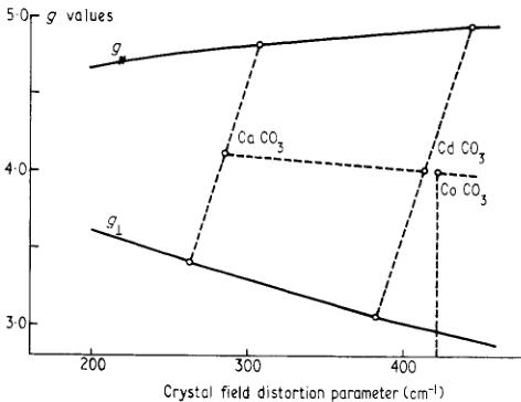
Paramagnetic resonance measurements have been made on \( Co^{2+} \) ions in two salts isostructural with \( CoCO_{3} \) . In otavite, \( CdCO_{3} \) , Borovic-Romanov et al (1967) found g parallel and perpendicular to the trigonal axis to be 3·06 and 4·94 respectively. Similar measurements of \( Co^{2+} \) in calcite, \( CaCO_{3} \) , by Antipin et al (1965) gave 3·41 and 4·82 respectively. A measure of the distortion from regularity of the oxygen octahedron in this structure is given by \( (3\cos^{2}\phi-1) \) , where \( \phi \) is the angle between the metal–oxygen bond and the trigonal axis. The calculation of this quantity requires, in addition to the cell dimensions, a knowledge of the oxygen positional parameter. This is not available for \( CdCO_{3} \) , but it is reasonable to assume that the \( CO_{3} \) group is unchanged in size between the three compounds. The distortion parameters are calculated as 0·0856, 0·0472, and 0·0448 for \( CaCO_{3} \) , \( CdCO_{3} \) and \( CoCO_{3} \) respectively. The full lines in figure 5 represent the values of \( g_{\parallel} \) and \( g_{\perp} \) as a function of the crystal field parameters computed for a spin–orbit coupling constant of 180 cm \( ^{-1} \) . The observed g values for

Figure 5. Curves used to estimate the crystal field distortion parameter in \( CoCO_{3} \) from g values obtained from EPR of \( Co^{2+} \) ions in \( CdCO_{3} \) and \( CaCO_{3} \) .
\( Co^{2+} \) ions in \( CaCO_{3} \) are indicated; the \( g_{\parallel} \) and \( g_{\perp} \) for each material do not correspond to exactly the same value of crystal field but it is possible to extrapolate from the mean values a probable crystal field parameter of \( 420\ cm^{-1} \) for \( CoCO_{3} \) itself. The corresponding coefficients of the eigenfunctions defined in equations (4) are
\[ b=0\cdot5403\quad a=-0\cdot7447\quad c=0\cdot3918. \]
In cobalt carbonate the exchange energy \( J_{1} \) , measured by the Néel temperature of 18·1 K, is much less than either the spin-orbit coupling or crystal field energies. The wavefunction of the ion in the antiferromagnetic salt can therefore be written to a good approximation as a linear combination of the \( \psi^{+} \) and \( \psi^{-} \) states given above. In this case the particular linear combination chosen determines the orientation of the antiferromagnetic moment. Both Alikhanov's study and the preliminary interpretation described in §3.2 above suggest that the magnetic moment is inclined at an angle of less than \( 90^{\circ} \) to the trigonal axis. Linear combinations were therefore chosen to give a range of inclination angles and
Table 1. Magnetic structure factors in Bohr magnetons per cobalt ion calculated for wavefunctions of the form \( x\psi^{+} + (y + iz)\psi^{-} \) for three values of the crystal field and three values of the inclination angle \( \beta \) . The angle \( \beta \) is given by \( \tan\beta = 2xzg_{\perp}/(x^{2} - z^{2})g_{\parallel} \) : \( y = 0.1z \) to give approximately the observed value for the spontaneous moment. The agreement index \( R = \Sigma|F_{obs} - F_{calc}|/\Sigma F_{obs} \) .
| hkl | sinθ/λ | Fobs | ΔFobs | Fcalc, Calculated magnetic structure factors | ||||||||
| 300 cm−1 | 420 cm−1 | 500 cm−1 | 500 cm−1 | |||||||||
| 46° | 68° | 90° | 46° | 68° | 90° | 46° | 68° | 90° | ||||
| 111 | 0·100 | 2·19 | 0·01 | 1·26 | 1·90 | 2·21 | 1·20 | 1·88 | 2·26 | 1·15 | 1·86 | 2·29 |
| 001 | 0·128 | 1·74 | 0·02 | 1·43 | 1·50 | 1·54 | 1·35 | 1·48 | 1·58 | 1·29 | 1·46 | 1·60 |
| 221 | 0·208 | 1·81 | 0·02 | 1·07 | 1·41 | 1·58 | 1·01 | 1·39 | 1·62 | 0·97 | 1·37 | 1·64 |
| 11T | 0·250 | 1·33 | 0·02 | 1·03 | 1·08 | 1·10 | 0·97 | 1·06 | 1·13 | 0·93 | 1·05 | 1·14 |
| 223 | 0·265 | 1·49 | 0·01 | 0·88 | 1·22 | 1·38 | 0·83 | 1·20 | 1·42 | 0·80 | 1·19 | 1·43 |
| 113 | 0·299 | 1·37 | 0·01 | 0·83 | 0·98 | 1·06 | 0·78 | 0·96 | 1·09 | 0·75 | 0·95 | 1·10 |
| 333 | 0·301 | 1·35 | 0·01 | 0·75 | 1·12 | 1·31 | 0·71 | 1·11 | 1·34 | 0·68 | 1·10 | 1·35 |
| 331 | 0·341 | 1·14 | 0·08 | 0·71 | 0·88 | 0·96 | 0·66 | 0·87 | 0·99 | 0·63 | 0·85 | 1·00 |
| 003 | 0·385 | 0·76 | 0·01 | 0·60 | 0·66 | 0·71 | 0·56 | 0·65 | 0·72 | 0·54 | 0·65 | 0·73 |
| 223 | 0·385 | 0·72 | 0·02 | 0·61 | 0·67 | 0·71 | 0·57 | 0·65 | 0·72 | 0·55 | 0·66 | 0·73 |
| 443 | 0·388 | 0·83 | 0·03 | 0·55 | 0·80 | 0·91 | 0·52 | 0·79 | 0·94 | 0·50 | 0·78 | 0·95 |
| 335 | 0·443 | 0·60 | 0·05 | 0·46 | 0·61 | 0·69 | 0·43 | 0·61 | 0·71 | 0·41 | 0·60 | 0·72 |
| 445 | 0·452 | 0·71 | 0·04 | 0·44 | 0·64 | 0·72 | 0·42 | 0·63 | 0·74 | 0·40 | 0·62 | 0·75 |
| 225 | 0·478 | 0·63 | 0·02 | 0·39 | 0·49 | 0·55 | 0·37 | 0·49 | 0·56 | 0·35 | 0·48 | 0·57 |
| 441 | 0·478 | 0·56 | 0·04 | 0·41 | 0·50 | 0·55 | 0·38 | 0·50 | 0·56 | 0·36 | 0·49 | 0·57 |
| 113 | 0·497 | 0·46 | 0·09 | 0·36 | 0·41 | 0·45 | 0·34 | 0·41 | 0·46 | 0·32 | 0·40 | 0·46 |
| 553 | 0·500 | 0·66 | 0·04 | 0·36 | 0·49 | 0·55 | 0·34 | 0·49 | 0·57 | 0·32 | 0·48 | 0·57 |
| 555 | 0·501 | 0·56 | 0·03 | 0·34 | 0·51 | 0·59 | 0·32 | 0·50 | 0·60 | 0·31 | 0·50 | 0·61 |
| 33T | 0·523 | 0·40 | 0·04 | 0·33 | 0·39 | 0·42 | 0·31 | 0·38 | 0·43 | 0·30 | 0·38 | 0·43 |
| 115 | 0·548 | 0·46 | 0·03 | 0·28 | 0·34 | 0·38 | 0·26 | 0·34 | 0·40 | 0·25 | 0·33 | 0·40 |
| 665 | 0·582 | 0·34 | 0·04 | 0·27 | 0·39 | 0·43 | 0·25 | 0·38 | 0·45 | 0·24 | 0·38 | 0·45 |
| 551 | 0·617 | 0·32 | 0·05 | 0·22 | 0·28 | 0·30 | 0·21 | 0·28 | 0·31 | 0·20 | 0·27 | 0·31 |
| 557 | 0·620 | 0·46 | 0·04 | 0·23 | 0·32 | 0·35 | 0·21 | 0·31 | 0·36 | 0·20 | 0·31 | 0·36 |
| 223 | 0·621 | 0·37 | 0·06 | 0·20 | 0·24 | 0·27 | 0·19 | 0·24 | 0·28 | 0·18 | 0·24 | 0·28 |
| 663 | 0·624 | 0·32 | 0·05 | 0·22 | 0·29 | 0·31 | 0·20 | 0·28 | 0·32 | 0·19 | 0·28 | 0·33 |
| 447 | 0·624 | 0·40 | 0·04 | 0·21 | 0·28 | 0·32 | 0·20 | 0·28 | 0·33 | 0·19 | 0·28 | 0·32 |
| 003 | 0·642 | 0·38 | 0·05 | 0·17 | 0·22 | 0·26 | 0·16 | 0·22 | 0·26 | 0·15 | 0·22 | 0·27 |
| Σ|Fobs−Fc| | 7·17 | 3·86 | 2·43 | 8·60 | 4·03 | 2·15 | 9·15 | 4·14 | 2·20 | |||
| R | 0·34 | 0·17 | 0·11 | 0·38 | 0·18 | 0·10 | 0·41 | 0·19 | 0·10 | |||
for each of these the magnetic scattering in the antiferromagnetic reflections was calculated for a range of crystal field parameters around that predicted. Some of the results are compared with the observed scattering amplitudes in table 1. It can be seen that, independent of the value of crystal field, the best agreement is obtained with equal contributions \( (1/\sqrt{2}) \) from the \( \psi^{+} \) and \( \psi^{-} \) states, that is with the moment in the basal plane. There is noticeably worse agreement for the lower crystal field value of \( 300\ cm^{-1} \) and slightly better agreement for the higher value of \( 500\ cm^{-1} \) , but the improvement is not sufficiently significant to justify changing the predicted crystal field value.
6. Calculation of the ferromagnetic moment
The effects on the wavefunction described in the previous section of the exchange interaction and an applied field parallel to the spontaneous moment were investigated. Two
possible model hamiltonians were tried. In the first, the exchange interaction was written as
\[ J_{1}\langle S_{i}\rangle[-0\cdot1\hat{S}_{X j}+0\cdot995\hat{S}_{Y j}]\qquad\mathrm{w i t h}\qquad J_{1}=-12\mathrm{c m}^{-1}. \]
X and Y are directions, lying in the basal plane perpendicular and parallel to a c-glide plane in the structure respectively. This model gives approximately the observed value for the spontaneous moment in zero field, but it can be seen from figure 1 that an applied field parallel to X increases the ferromagnetic component at a much faster rate than that observed by Borovik-Romanov et al. This shows that the magnetic moment direction is coupled more strongly to the lattice than this model would suggest. In the second model it is proposed that the orbital moment direction is coupled to a symmetry direction of its local environment by a term of the form \( \delta\hat{L}_{y} \) , which favours a moment lying perpendicular to the trigonal axis in a mirror plane of the local octahedron. The exchange energy is then assumed to be of the form \( J_{1}\langleS_{i}\rangle\cdot\hat{S}_{j} \) where i and j label antiferromagnetically coupled neighbours. Because octahedra around antiferromagnetically coupled ions are rotated oppositely by a small angle away from the glide plane, the hamiltonian leads to an antiferromagnetic structure with a small spontaneous moment. A value of \( \delta \) of \( -32~cm^{-1} \) was selected to give approximately the observed moment in zero field. The variation of moment with applied field was then found to be in much better agreement with experiment (figure 1). The lowest energy eigenvectors of this hamiltonian in zero field and for the two field values of the experiment are shown in table 2.
Table 2. The lowest energy eigenvectors of the hamiltonian proposed for the \( Co^{2+} \) ion in cobalt carbonate. The eigenvectors given are for zero magnetic field and the two field values of the experiment.
| Applied field parallel to [1T0] kOe | b | ψ+ a | c | c | ψ− a | b |
| 0 | 0·3652 | -0·5287 | 0·2951 | 0·0326 | -0·0555 | 0·0370 |
| 0 | -0·0019 | 0·0027 | 0·2933 | -0·5258 | 0·3634 | |
| 3·6 | 0·3652 | -0·5287 | 0·2951<|/ref|> | 0·0355 | -0·0607 | 0·0407 |
| 0 | -0·0018 | 0·0026 | 0·2930 | -0·5252 | 0·3629 | |
| 14·6 | 0·3651 | -0·5287 | 0·2952 | 0·0445 | -0·0773 | 0·0523 |
| 0 | -0·0015 | 0·0022 | 0·2918 | -0·5230 | 0·3614 |
7. Comparison of observed and calculated scattering
The three wavefunctions given in table 2 have been used to predict the scattering which should be observed in the experiments of §3.2 and §3.3. The agreement obtained for the antiferromagnetic scattering is quite good, as shown by table 3. Similarly there is fair agreement between the observed and calculated ferromagnetic scattering at the lower applied field (table 4). On the other hand, the results for the high field experiments are in much less good agreement with the model.
To facilitate comparison between the three sets of results, they have been normalized to unit magnetic moment and, in the case of the antiferromagnetic scattering, divided by the square root of the effective domain factors. This procedure enables them all to be plotted as form factors and compared directly with one another. The results are given
Table 3.
| hkl | sin θ/λ | Magnetic structure factors | Normalized form factors | ||||
| Calc. | Obs. | Std dev. | Calc. | Obs. | Std dev. | ||
| 111 | 0·100 | 2·32 | 2·19 | 0·01 | 0·924 | 0·872 | 0·004 |
| 001 | 0·128 | 1·62 | 1·74 | 0·02 | 0·884 | 0·948 | 0·011 |
| 221 | 0·208 | 1·66 | 1·81 | 0·02 | 0·729 | 0·796 | 0·009 |
| 11T | 0·250 | 1·16 | 1·33 | 0·02 | 0·649 | 0·741 | 0·011 |
| 223 | 0·265 | 1·46 | 1·49 | 0·01 | 0·617 | 0·629 | 0·004 |
| 113 | 0·299 | 1·12 | 1·37 | 0·01 | 0·550 | 0·673 | 0·005 |
| 333 | 0·301 | 1·38 | 1·35 | 0·01 | 0·550 | 0·538 | 0·004 |
| 331 | 0·341 | 1·07 | 1·14 | 0·08 | 0·474 | 0·530 | 0·037 |
| 003 | 0·385 | 0·75 | 0·76 | 0·01 | 0·406 | 0·414 | 0·005 |
| 223 | 0·385 | 0·75 | 0·72 | 0·02 | 0·406 | 0·394 | 0·011 |
| 443 | 0·388 | 0·97 | 0·83 | 0·03 | 0·394 | 0·338 | 0·012 |
| 335 | 0·443 | 0·73 | 0·60 | 0·05 | 0·318 | 0·259 | 0·022 |
| 445 | 0·452 | 0·77 | 0·71 | 0·04 | 0·315 | 0·287 | 0·016 |
| 225 | 0·478 | 0·58 | 0·63 | 0·02 | 0·279 | 0·299 | 0·009 |
| 441 | 0·478 | 0·58 | 0·56 | 0·04 | 0·279 | 0·267 | 0·019 |
| 113 | 0·497 | 0·48 | 0·46 | 0·09 | 0·267 | 0·259 | 0·051 |
| 553 | 0·500 | 0·59 | 0·66 | 0·04 | 0·251 | 0·279 | 0·017 |
| 555 | 0·501 | 0·63 | 0·56 | 0·03 | 0·251 | 0·223 | 0·012 |
| 33T | 0·523 | 0·44 | 0·40 | 0·04 | 0·239 | 0·215 | 0·021 |
| 115 | 0·548 | 0·41 | 0·46 | 0·03 | 0·215 | 0·239 | 0·016 |
| 665 | 0·582 | 0·47 | 0·34 | 0·04 | 0·187 | 0·135 | 0·015 |
| 551 | 0·617 | 0·32 | 0·32 | 0·05 | 0·159 | 0·155 | 0·024 |
| 557 | 0·620 | 0·38 | 0·46 | 0·04 | 0·159 | 0·191 | 0·016 |
| 223 | 0·621 | 0·29 | 0·32 | 0·06 | 0·167 | 0·179 | 0·033 |
| 663 | 0·624 | 0·34 | 0·32 | 0·05 | 0·147 | 0·139 | 0·022 |
| 447 | 0·624 | 0·34 | 0·40 | 0·04 | 0·151 | 0·175 | 0·018 |
| 003 | 0·642 | 0·28 | 0·38 | 0·05 | 0·151 | 0·207 | 0·027 |
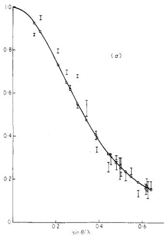
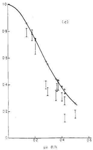
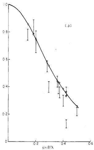
in tables 3 and 4 and illustrated in figure 6. In each case the solid curve is the isotropically averaged form factor deduced for the wavefunctions of table 2; it is substantially the same for the three functions. Examination of figure 6 shows that, whereas the observed scattering in the antiferromagnetic reflections falls off less rapidly with angle than the calculated form factor, the ferromagnetic scattering falls off more rapidly. These general results might be expected if there is significant moment transferred to the ligands due to covalency.
Covalency will lead to a more swiftly varying antiferromagnetic moment distribution because of cancellation of oppositely directed moment around the ligand atoms. The ferromagnetic moment, on the other hand, is spread out onto the ligands: the moment distribution varies less swiftly than that of the free ion and the form factor falls off more rapidly with \( \sin\theta/\lambda \) .
The experimental points in figure 6 vary significantly from smooth curves and indicate a greater degree of anisotropy in the moment distribution than can be accounted for by the aspherical contributions to the calculated ionic form factors. If the major part of the difference between the observed and calculated form factors arises from covalency then the difference between observed and calculated magnetic moment distributions should show significant features associated with the cobalt–oxygen interatomic vectors. Figures 7 and 8 show the \( [1\overline{1}0] \) projections of the normalized difference densities calculated from the difference between the observed and calculated normalized form factors.
| Table 4. Comparison of observed and calculated scattering by the ferromagnetic moment in CoCo2. To allow for the effect of temperature on the aligned moment the scattering calculated from the wavelengths of 2 has been multiplied by the ratio M0/Mw where M0 is the moment parallel to [110] calculated from the wavelengths appropriate to OK] and M0 is the ferromagnetic moment observed at 42 K. The units of the magnetic structure factors are \( \mu \) B per cobalt ion. | |||||||||||
| HKJ | Field parallel to [110] 3 kOe | ||||||||||
| Magnetic structure factors | |||||||||||
| 110 | 0.141 | Calc. | Obs. | Sd dev. | Calc. | Obs. | Sd dev. | Calc. | Magnetic form factors | ||
| 112 | 0.182 | 0.217 | 0.013 | 0.078 | 0.084 | 0.054 | 0.037 | 0.300 | 0.015 | 0.758 | 0.778 |
| 222 | 0.201 | 0.207 | 0.203 | 0.079 | 0.073 | 0.088 | 0.283 | 0.257 | 0.020 | 0.744 | 0.068 |
| 320 | 0.282 | 0.159 | 0.153 | 0.076 | 0.055 | 0.044 | 0.219 | 0.154 | 0.010 | 0.575 | 0.040 |
| 332 | 0.295 | 0.154 | 0.111 | 0.056 | 0.040 | 0.044 | 0.211 | 0.135 | 0.012 | 0.554 | 0.035 |
| 324 | 0.357 | 0.123 | 0.122 | 0.040 | 0.044 | 0.169 | 0.123 | 0.112 | 0.015 | 0.443 | 0.203 |
| 224 | 0.365 | 0.121 | 0.116 | 0.040 | 0.039 | 0.064 | 0.165 | 0.145 | 0.010 | 0.433 | 0.238 |
| 112 | 0.372 | 0.120 | 0.108 | 0.040 | 0.034 | 0.064 | 0.165 | 0.145 | 0.012 | 0.433 | 0.339 |
| 444 | 0.401 | 0.107 | 0.082 | 0.010 | 0.038 | 0.030 | 0.048 | 0.119 | 0.030 | 0.389 | 0.330 |
| 114 | 0.422 | 0.101 | 0.103 | 0.003 | 0.365 | 0.037 | 0.003 | 0.137 | 0.016 | 0.010 | 0.360 |
| 330 | 0.422 | 0.092 | 0.037 | 0.003 | 0.332 | 0.013 | 0.003 | 0.127 | 0.059 | 0.010 | 0.334 |
| 222 | 0.520 | 0.072 | 0.060 | 0.028 | 0.260 | 0.022 | 0.003 | 0.100 | 0.067 | 0.010 | 0.262 |
| 0.026 | 0.118 | ||||||||||
| I/kg = -R = 0.09 | |||||||||||


Figure 6. Observed and calculated form factors for \( Co^{2+} \) in \( CoCO_{3} \) . The vertical bars give the observed points and the open circles the calculated values. The full curves are the isotropically averaged theoretical form factors. (a) is obtained from the antiferromagnetic scattering in zero applied field. (b) and (c) are for the ferromagnetic scattering in fields of 3·6 and 14·6 kOe respectively.

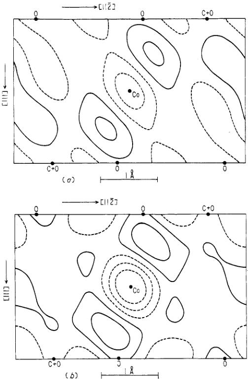
Figure 7. Normalized difference densities obtained from the ferromagnetic scattering (a) in a field of \( 3.6 \, kOe \) , (b) in a field of \( 14.6 \, kOe \) . The contour intervals are \( 0.06 \, \AA^{-2} \) , negative contours are shown by broken lines. The difference density has been averaged over a square of edge \( 0.40 \, \AA \) to reduce series termination effects. The standard deviation of the density is approximately one contour interval.
Figures 7(a) and (b) show the same general features—a negative difference density near the cobalt site indicating an expansion of the moment distribution and significant areas of positive difference density associated with the oxygen ligands. These difference density distributions are remarkably similar to those obtained for \( MnCO_{3} \) under the same conditions (Brown and Forsyth 1967). As in \( MnCO_{3} \) , the position of the oxygen atom projected over the carbon atom is associated with a small negative difference density which indicates an opposite polarization associated with carbon in the carbonate group. Additionally, there is a small but probably significant difference between the difference densities at high and low fields, suggesting that the spontaneous and the field induced distributions are not identical. In this again the results are similar to those for

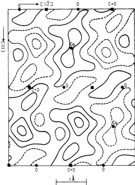
Figure 8. Normalized difference density obtained from the antiferromagnetic scattering. The area of the map is twice that of figure 7. Nodal points are marked as solid squares. The contour interval is \( 0.03 \AA^{-2} \) , otherwise the details are as in figure 7.
manganese carbonate. The distribution of field induced moment seems to be more strongly affected by covalency than that of the spontaneous moment.
Figure 8 is of necessity very different from figure 7, since it represents an antiferromagnetic distribution. The projection covers twice the area of those in figure 7 so that the antiferromagnetic symmetry is easily seen and the nodal points are indicated.
The significant features of figure 8 can be qualitatively described as showing an elongation of the \( Co^{2+} \) moment towards the planes containing the anions, with a corresponding contraction in the 111 plane passing through the cation. The extent of the elongation is effectively curtailed by the antiferromagnetic structure.
8. Discussion
The surprising result of this study has been the conclusion that in \( CoCO_{3} \) the cobalt moment lies in the basal plane. This result is only obtained when rather detailed calculations of the scattering by \( Co^{2+} \) ions having physically reasonable wavefunctions are made. It should be pointed out again that both the previous study by Alikhanov (1961) and our own preliminary investigation, in which an arbitrary form factor was allowed,
gave a significantly different conclusion. This result may call into doubt magnetic structure determinations based on rather few data and uncertain ionic form factors.
The data we have obtained in the present investigation is regrettably less good than that used in the similar study of \( MnCO_{3} \) . The accuracy was limited both by the small size of the only available crystals and by the presence of extinction. For this reason, no attempt has been made to refine our theoretical model beyond that described in §5 and §6. The effects of possible admixture of higher states such as \( {}^{4}P \) and the undoubted existence of a zero-point spin deviation in the antiferromagnetic case will predict scattering differences smaller than the observational uncertainties. Similarly, we feel that a detailed calculation of the effects of covalency would not be justified.
We have however shown that, using the magnetization density approach, we can calculate the effects of orbital scattering in the relatively simple case of a first group transition metal ion. After orbital scattering is allowed for, our results show great similarity to those obtained for \( MnCO_{3} \) . These have in turn been very successfully interpreted by Lingard and Marshall (1969) and the present study must therefore add weight to the validity of their model and in particular to the exchange polarization of the carbonate group. Both investigations suggest a difference between the spatial distribution of the spontaneous and field induced moments, but no satisfactory explanation for this effect has yet been given.
Acknowledgments
We are indebted to Dr N Y Ikornikova and Dr A N Lobachev of the Institute of Crystallography, USSR Academy of Science, Moscow who provided us with single crystals of \( CoCO_{3} \) . The program of which this research forms a part is supported by generous grants from the Science Research Council and the United Kingdom Atomic Energy Authority, to whom we express our thanks.
References
Alikhanov R A 1961 Sov. Phys.-JETP 12 1029
Anderson P W 1959 Phys. Rev. 115 2
Antipin A A. Vinokwov V M and Zaripov M M 1965 Sov. Phys.-Solid St. 6 1718
Borovik-Romanov A S and Orlova M P 1957 Sov. Phys.-JETP 4 531
Borovik-Romanov A S and Ozhogin V I 1961 Sov. Phys.-JETP 12 18
Brown P J 1970 Thermal Neutron Diffraction ed B T M Willis (Oxford: University Press) p 179
Brown P J and Forsyth J B 1967 Proc. Phys. Soc. 92 125
Dzyaloshinskii I 1957 Sov. Phys.-JETP 5 1259
Edmonds A D 1957 Angular Momentum in Quantum Mechanics (Princeton: University Press)
Kaplan T A 1964 Phys. Rev. 136 A1636
Lingard P A and Marshall W 1969 J. Phys. C: Solid St. Phys. 2 276
Moriya T 1960 Phys. Rev. 120 91
Steinsvoll O et al 1967 Phys. Rev. 1612 499
Trammell G T 1953 Phys. Rev. 92 1387
Watson R E 1959 Tech. rep. no. 2, Solid St. Molec. Theory Group, MIT Cambridge Mass. USA
Watson R E and Freeman A J 1961 Acta crystallogr. 14 27
Zachariasen W H 1945 The Theory of Diffraction of X-rays in Crystals (New York: Wiley)
—— 1967 Acta crystallogr. 23 558
 p10_0.jpg
 p15_0.jpg
 p15_1.jpg
 p15_2.jpg
 p16_0.jpg
 p17_0.jpg
 p3_0.jpg
 p4_0.jpg
 p6_0.jpg
 p9_0.jpg