| Transition Temperature | 67 K |
|---|---|
| Propagation Vector | k1 (0, 0, 0) |
| Parent Space Group | P42/mnm (#136) |
| Magnetic Space Group | P42'/mnm' (#136.499) |
| Magnetic Point Group | 4'/mm'm (15.4.56) |
| Lattice Parameters | 4.8736 4.8736 3.3000 90.0000 90.0000 90.0000 |
|---|---|
| DOI | 10.1139/p10-081 |
| Reference | Z. Yamani, Z. Tun and D.H. Ryan, Canadian Journal of Physics (2010) 88 771-797. |
| Label | Element | Mx | My | Mz | |M| |
|---|---|---|---|---|---|
| Mn1 | Mn | 0.0 | 0.0 | 4.6 | 4.60 |
Neutron scattering study of the classical antiferromagnet MnF_{2}: a perfect hands-on neutron scattering teaching course \( ^{1} \)
Z. Yamani, Z. Tun, and D.H. Ryan
Abstract: We present the classical antiferromagnet \( MnF_{2} \) as a perfect demonstration system for teaching a remarkably wide variety of neutron scattering concepts. The nature of antiferromagnetism and the magnetic Hamiltonian in this classical antiferromagnet are discussed. The transition temperature to the Neel state, the value of magnetic moment in the ordered state, the critical scattering close to the phase transition, spin waves associated with the ordering of the moments, as well as their dispersion and temperature dependences are determined experimentally. Parameters such as the Neel transition temperature and exchange coupling constants obtained from the experiments agree reasonably well with the previously published data. In addition, details of how an inelastic neutron scattering experiment is performed by means of triple-axis spectroscopy are provided.
PACS Nos: 72.10.Di, 71.70.Ej, 71.70.Gm, 78.70.Nx
Résumé : Nous présentons l’antiferromagnétique \( MnF_{2} \) comme un exemple pédagogique parfait pour montrer une foule de concepts en diffusion de neutrons. Nous analysons la nature de l’antiferromagnétisme et le hamiltonien magnétique de ce spécimen antiferromagnétique. Nous déterminons expérimentalement la température de transition de Néel, la valeur du moment magnétique dans l’état ordonné, la diffusion critique près de la transition de phase, les ondes de spin associées à la mise en ordre des moments, aussi bien que leur dispersion et leur dépendance en température. Les paramètres obtenus ici, comme la température de transition de Néel et les constantes du couplage d’échange sont en assez bon accord avec les valeurs déjà publiées. De plus, nous présentons de façon détaillée la diffusion de neutrons à l’aide d’un spectrographe à trois axes.
[Traduit par la Rédaction]
1. Introduction
This article is an outcome of a graduate level course offered by the Physics Department of McGill University on experimental techniques in condensed matter physics. As one of the modules of the course, the students travel to Chalk River for a hands-on demonstration experiment at NRU, studying a single crystal of \( MnF_{2} \) . The topics that will be touched upon in the article are the ones that the students are exposed to during the experiment, and the data presented here were taken by the graduate students who attended the course.
This article is not meant to be a full account of any of
Received 27 August 2010. Accepted 4 October 2010. Published on the NRC Research Press Web site at cjp.nrc.ca on 3 November 2010.
Z. Yamani \( ^{2} \) and Z. Tun. National Research Council, Canadian Neutron Beam Centre, Chalk River, ON K0J 1J0, Canada. D.H. Ryan. Department of Physics and Centre for the Physics of Materials, McGill University, 3600 University Street, Montreal, QC H3A 2T8, Canada.
\( ^{1} \) Special issue on Neutron Scattering in Canada. \( ^{2} \) Corresponding author (e-mail: zahra.yamani@nrc.gc.ca). these topics. Rather, it is intended to convey the breadth of the topics we manage to cover within this 3-day crash course, and thus demonstrate the educational aspect of NRU, one of the functions this 50+ year-old reactor continues to provide for the benefit of Canada.
1.1 Neutron scattering
Condensed matter physics has benefited tremendously from both elastic and inelastic neutron scattering techniques, almost from the beginning of neutron scattering more than half a century ago. These techniques were developed in 1940s and the 1950s by C. Shull at Oak Ridge and B. Brockhouse at Chalk River, who shared the 1994 Nobel Prize in physics for their groundbreaking work. Since then, neutron scattering has been used to study a wide variety of materials.
The main reasons for wide application of neutron scattering arise from the unique physical properties of the neutron itself. It has zero electric charge hence does not interact with the electrons in a way that electromagnetic radiation does. Neutrons interact with the atomic nuclei in matter via the nuclear force, which is extremely short-ranged. Hence, neutrons only weakly perturb the system under study; i.e., neu-
trons are both nondestructive and highly penetrating. This allows an investigation of the interior of materials and obtaining the bulk response of the system. Since neutrons with wavelengths similar to interatomic distances are readily available, structural measurements over distances from the shortest hydrogen bonds to macromolecules are possible. Also, since the energies of the neutrons with such wavelengths match the energy scales of many condensed matter systems, it is possible to use them to probe the dynamics of the system. Excitations that can be studied via neutron scattering range in energy from a few milli-electron volts (meV) to a fraction of an electron volt. In addition, since the neutron has a magnetic moment, it interacts with unpaired electrons in solids. By coincidence, the cross-sections for the magnetic and nuclear interactions are of similar magnitudes. Thus, the neutron is the probe of choice for investigating magnetic materials, as it often provides crucial information about the magnetic properties of the system that cannot be obtained by other techniques.
The description of magnetic neutron scattering presented here is necessarily brief. For a more extensive introduction to the general techniques see refs. 1 and 2. Polarized neutron methods have been discussed by Williams [3], while Lovesey provides a more comprehensive theoretical text [4]. References 5 and 6 are excellent detailed texts on the experimental aspects of neutron scattering. Other useful texts on different aspects of neutron scattering are listed in refs. 7–11.
The very first concept the students are introduced to is the following: In a neutron scattering experiment, the quantity we ultimately measure is the time and spatial Fourier transform of the correlation function of the objects that cause scattering, the so-called scattering function, \( S(\mathbf{Q}, \omega) \) . For magnetic neutron scattering, this quantity is the Fourier transform of the time-dependent correlation function of magnetic moments (either due to spin only or to the total angular momentum). The partial differential cross-section, \( \mathrm{d}^{2}\sigma/(\mathrm{d}\Omega\mathrm{d}E_{f}) \) , per solid angle \( \Omega \) , per unit energy E, is given by
\[ \mathrm{d}^{2}\sigma\mathrm{d}E_{f}=\frac{k_{f}}{\kappa_{i}}\mathrm{e}^{-2W(\mathbf{Q})}\sum_{\alpha\beta}\left(\delta_{\alpha\beta}-\widehat{Q}_{\alpha}\widehat{Q}_{\beta}\right)S_{\mathrm{mag}}^{\alpha\beta}(\mathbf{Q},\omega) \quad (1) \]
where
\[ \begin{align*}S_{\mathrm{mag}}^{\alpha\beta}(\boldsymbol{Q},\omega)=\left(\frac{\gamma^{\prime}n r_{0}g}{2}\right)^{2}\int\mathrm{d}t\mathrm{e}^{-\mathrm{i}\omega t}\\ \times\sum_{f}f_{i}^{*}(\boldsymbol{Q})f_{f}(\boldsymbol{Q})\mathrm{e}^{\mathrm{i}\boldsymbol{Q}\cdot(\boldsymbol{r}_{f}-\boldsymbol{r}_{i})}\langle S_{i}^{a}(0)S_{f}^{b}(t)\rangle\quad(2)\end{align*} \]
with the summation over Cartesian directions, \( \gamma_{n}=1.913 \) is the gyromagnetic ratio of the neutron, \( r_{0} \) is the classical electron radius, \( g \sim 2 \) Lande factor, \( \boldsymbol{k}_{i} \) ( \( \boldsymbol{k}_{f} \) ) is the incident (scattered) neutron wavevector, \( Q=k_{i}-k_{f} \) the momentum transfer in the scattering process, \( \omega \) is the energy transfer (assuming the reduced Planck constant \( \hbar=1 \) ), \( f(\boldsymbol{Q}) \) is the magnetic form factor, discussed in more detail in Sect. 1.3, \( \mathrm{e}^{-2W(\boldsymbol{Q})} \) is the Debye–Waller factor (DWF) \( ^{3} \) , and \( S_{\mathrm{mag}}^{\alpha\beta}(\boldsymbol{Q}, \omega) \) Fig. 1. The magnetic intensity is zero when the magnetic moment and the scattering vector (momentum transfer in a scattering event) are parallel to each other. The diagram shows the condition for elastic scattering.

is the magnetic scattering function, the space and time Fourier transform of the time-dependent correlation function of magnetic moments. The \( (\delta_{\alpha\beta}-\widehat{\boldsymbol{Q}}_{\alpha}\widehat{\boldsymbol{Q}}_{\beta}) \) term in the cross-section indicates that only the components of spin perpendicular to the momentum transfer Q are probed by neutrons. In other words, the measured intensity is proportional to \( \sin^{2}\alpha \) , where \( \alpha \) is the angle between the magnetic moment and the momentum transfer, as depicted in Fig. 1.
The magnetic scattering function \( S_{\mathrm{mag}}^{\alpha\beta}(\boldsymbol{Q}, \omega) \) is also related to the imaginary part of the generalized dynamical spin susceptibility \( \chi'(\boldsymbol{Q}, \omega) \) , through the fluctuation-dissipation theorem [12],
\[ S_{\mathrm{m a g}}^{\alpha\beta}(\boldsymbol{Q},\omega)\propto[n(\omega)+1]\chi_{\alpha\beta}^{\prime\prime}(\boldsymbol{Q},\omega) \quad (3) \]
where
\[ [n(\omega)+1]=\frac{1}{1-\mathrm{e}^{-\hbar\omega/k_{\mathrm{B}}T}} \]
accounts for the Bose factor, where \( k_{B} \) is the Boltzmann constant.
We will now give a brief description of magnetic order and magnetic excitations. To keep our discussion simple, we will only consider a special class of materials known as co-linear magnets.
In the lowest energy state of a long-range ordered magnet, the magnetic moments of all ions point along a specific direction (let us assume this direction is along z-axis), which is defined by the magnetic structure of the lattice. In an antiferromagnet (more common in nature than ferromagnets), orienting the nearest-neighbour moments anti-parallel to each other leads to the lowest-energy configuration, while the parallel configuration is favoured in a ferromagnet. In general, the magnetic moment of an ion is derived from both the spin and the orbital angular momenta of its unpaired electrons. Here we consider magnetic order in \( MnF_{2} \) , where the situation is simpler: the moment is due solely to
the spin-angular momentum of unpaired electrons, as discussed in the next section.
One might expect that the first excited state would be created by reversing the sign of a single magnetic moment, but this simple configuration turns out to be highly energetic since it involves the breaking of two antiferromagnetic bonds (see the lower part of Fig. 2a). For a relatively high spin ion such as \( Mn^{2+} \) , excited states with much lower energy can be constructed by having the spins at each site lower their \( S_{z} \) component by one unit, while acquiring an xy-component (clearly not possible in a spin-1/2 system). However, it is more energetically favourable that the change in spin angular momentum is shared by all of the spins; i.e., instead of one moment reversing its sign, with the newly acquired xy-components it is now possible for all the moments to precess about their equilibrium positions at an angular frequency establishing a spin wave with a repeat distance of several lattice spacings, as shown in Fig. 2b. For a system of N ions, each ion carries a share of \( \hbar/N \) in the reduction of \( S_{z} \) . These quantized spin waves are called magnons, the quantization arising from the fact that \( S_{z} \) can only change by integral multiples of \( \hbar \) . In the absence of easy axis anisotropy, magnons have exceedingly small energies in the limit of infinite wavelengths. Such excitations are called Goldstone modes. In the presence of anisotropy (e.g., as is the case for \( MnF_{2} \) ), an energy gap will develop at the zone centre of the magnetic Brillouin zone.
A neutron scattering experiment can be performed, measuring the scattered neutrons either elastically or inelastically, to investigate the nature of magnetic order. In an elastic experiment, the incident and scattered neutron energies are set to be equal to each other, and we measure \( S(\mathbf{Q}, \omega = 0) \) . Thereby, as a consequence of the time Fourier transform, the correlations we probe correspond to infinite time, i.e., the static property of the sample. From the observed magnetic scattering pattern, the (time-independent) magnetic structure can then be determined. In addition, as seen from (1), since the observed scattering is only nonzero when the magnetic moment has a component perpendicular to the scattering wavevector, one can often gain information about the orientation of the magnetic moment in the system under study. For a system where the magnetic moments are ordered into a long-range periodic pattern, the scattering will appear as delta functions at the wavevectors corresponding to magnetic Bragg reflections. For a system where only short magnetic correlation exist, the observed peaks will have a finite width. For such systems, the spatial extent of the correlations can be investigated by measuring the peak width in reciprocal space, as the correlation length is inversely proportional to the width, after deconvolving the intrinsic resolution function of the instrument (see Sect. 2.6).
In an inelastic experiment, the incident and scattered neutron energies are different, and hence one is able to study the spin dynamics of the system from such measurements. In a long-range magnetically ordered system, the collective magnetic excitations are spin waves, as explained above. These excitations and their dependence on wavevector can easily be measured by neutrons. From the observed dependence of the excitation energy on wavevector (dispersion relations), information about fundamental properties of the magnetic interactions, such as exchange coupling constants
Fig. 2. (a) In the lowest state, all moments are pointing along a specific direction (antiparallel to one another in an antiferromagnet). The first excited state is when the total spin is reduced by one. This can be achieved by the reversal of only one moment as shown in (a). However, it is more energetically favourable if the change is shared by all the moments, i.e., all the moments precess about their equilibrium positions, as shown in (b).
(a)

(b)

and their anisotropy, can be determined. Furthermore, information about the lifetime of magnetic excitations can be obtained from a study of the energy width of the observed excitation peaks. Such elastic and inelastic information is often crucial in studying microscopic magnetic structures and the magnetic fluctuations that underpin macroscopic magnetic phenomena in materials.
1.2 Antiferromagnetism in \( MnF_{2} \)
\( MnF_{2} \) is a classical antiferromagnetic insulator with a Neel transition to an AF state at \( T_{N} \approx 67 K \) [13–15]. Similar to other transition metal difluorides, \( MnF_{2} \) has [16] a tetragonal structure (space group \( P4_{2}/mnm \) ) with lattice constants \( a = b = 4.873 \AA \) , and \( c = 3.130 \AA \) . The tetragonal structure has a large compression along the c-axis with c/a of about two thirds. The \( Mn^{2+} \) ions occupy the body centre positions at \( (0, 0, 0) \) and \( (0.5, 0.5, 0.5) \) . The F ions are located in noncentrosymmetric positions between the \( Mn^{2+} \) ions at \( (x, x, 0) \) , \( (-x, -x, 0) \) , \( (0.5 + x, 0.5 - x, 0.5) \) , and \( (0.5 - x, 0.5 + x, 0.5) \) with \( x \approx 0.3 \) (see Table 1). The \( MnF_{2} \) unit cell is shown in Fig. 3.
\( MnF_{2} \) contains \( Mn^{2+} \) and \( F^{-} \) ions. \( Mn^{2+} \) is a transition metal ion with the half-filled electronic configuration 3d \( ^{5} \) . Many properties of compounds made of transition metal ions, including magnetic ordering and their colour, are due to the partially filled d-orbitals of these ions [18–20]. Since the fluoride ion is in the full 2p \( ^{6} \) electronic state, it does not have any unpaired electrons, and hence it does not directly participate in the magnetic state of the compound, and the transition to an AF state below \( T_{N} \) is due to the \( Mn^{2+} \) ion.
The electronic configuration of the ground state of a free ion can be predicted by the Hund's rules [21]. According to these rules, the equivalent electrons of the last shell of a free ion fill available orbitals in that shell such that first the total spin angular momentum, \( S = \Sigma_{i}s_{i} \) (sum over all electrons), is maximized as allowed by the Pauli principle, then the total orbital angular momentum \( L = \Sigma_{i}l_{i} \) is maximized. And finally, J, the total angular momentum is defined as \( J = |L - S| \) for a half-filled or less, and \( J = L + S \) for a shell that is more
Table 1. The atomic positions in the \( MnF_{2} \) nuclear unit cell (space group \( P4_{2}/mnm \) ) with lattice constants \( a=b=4.873\mathring{A} \) , and \( c=3.130\mathring{A} \) [16]. The nuclear scattering length for Mn is -3.73 fm and for F is 5.56 fm [17].
| x | y | z | Atoms per unit cell | |
| Mn | 0 | 0 | 0 | 1/8 |
| Mn | 0 | 0 | 1 | 1/8 |
| Mn | 0 | 1 | 0 | 1/8 |
| Mn | 0 | 1 | 1 | 1/8 |
| Mn | 1 | 0 | 0 | 1/8 |
| Mn | 1 | 0 | 1 | 1/8 |
| Mn | 1 | 1 | 0 | 1/8 |
| Mn | 1 | 1 | 1 | 1/8 |
| Mn | 0.5 | 0.5 | 0.5 | 1 |
| F | 0.305 | 0.305 | 0 | 1/2 |
| F | 0.305 | 0.305 | 1 | 1/2 |
| F | 0.695 | 0.695 | 0 | 1/2 |
| F | 0.695 | 0.69 | 1 | 1/2 |
| F | 0.805 | 0.195 | 0.5 | 1 |
| F | 0.195 | 0.805 | 0.5 | 1 |
Fig. 3. The tetragonal nuclear unit cell of \( MnF_{2} \) is shown. The manganese ions (small red spheres; dark grey in the print version) are located at the corners and the body centre positions. The fluoride ions (large blue spheres; light grey) are located at non-centrosymmetric positions between the \( Mn^{2+} \) ions. The unpaired electrons of \( Mn^{2+} \) ions, ordered antiferromagnetically, are shown with red arrows. The AF magnetic structure can be described by two sublattices (both shown as outlines) of \( Mn^{2+} \) ions ( \( Mn_{1} \) and \( Mn_{2} \) ) with their moments pointing along the c-axis and antiparallel to one another. The arrangement of the fluoride ions around each \( Mn^{2+} \) ion is identical but rotated by \( 90^{\circ} \) about the c-axis. The crystal field at each \( Mn^{2+} \) ion is mainly octahedral.

than half-filled. Hund's rules can be understood by considering the Coulomb repulsion between the electrons and the Pauli exclusion principle, which states that two electrons with the same spin state are forbidden to occupy the same orbital. Since the total spin angular momentum S has to be maximal, electrons first occupy separate orbitals, while having the same spin state. This way, the Coulomb repulsion is minimized since electrons will be as far as possible from one another. For the \( Mn^{2+} \) ion, according to Hund's rules, each of the five d-orbitals is occupied with one of the five electrons. The spins of all five electrons are aligned in the same direction, thus leading to a high spin state of S=5/2 for this ion. Since there is an electron in each of the five d-orbitals (l=-2,-1,0,1,2), the total orbital angular momentum is zero, L=0, and therefore J=5/2 for the ground state. This indicates that the magnetic moment of the \( Mn^{2+} \) ion is due solely to its spin angular momentum. This is in fact experimentally verified, since the observed magnetic moment and the spin magnetic moment are identical.
The magnetic properties of materials cannot be understood in terms of free-ion properties alone, and the interaction of the ions with one another and their surrounding environment needs to be included \( [12, 21] \) . Here, we first briefly consider the interaction of the ion with the electric field generated by the neighbouring ions in the crystal (crystal field) and then consider the magnetic interaction between the ions.
The atomic levels of a metallic ion when surrounded by negatively charged ions (ligands) in a crystal depend on the local environment around the ion. A free ion has spherical symmetry, and its d-orbitals all have the same energy (they are degenerate); in a crystal, the spherical symmetry of the ion is broken, thus the degeneracy of the d-orbitals is lifted. The symmetry of the local environment determines the pattern of splitting, whereas the size of the splitting depends on the type of ligand.
The angular dependence of the five d-orbitals is shown in Fig. 4. In an octahedral crystal field (where the magnetic ion is at the centre of an octahedron made by the six surrounding ligands, as is the case with Mn in \( MnF_{2} \) ), electronic orbitals of \( Mn^{2+} \) (three \( t_{2g} \) orbitals) that have smaller overlap with the orbitals from the ligands, will have a lower energy than the orbitals (two \( e_{g} \) orbitals) with lobes directed towards the ligands, as shown in Fig. 4. This is due to the Coulomb repulsion between the electrons from the ligands and the magnetic ion. For this local symmetry, the amount of energy shift is calculated to be \( -2\Delta/5 \) and \( 3\Delta/5 \) for the \( t_{2g} \) and the \( e_{g} \) orbitals, respectively, where \( \Delta \) is the splitting of the d-orbitals in an octahedral field [12, 18–20]. For compounds with weak (strong) crystal field, the ground state of
Fig. 4. The angular dependence of the d-orbitals. The three similar orbitals (of symmetry \( t_{2g} \) ) \( d_{xy} \) , \( d_{yz} \) , and \( d_{xz} \) consist of four lobes of high electron density in between the principal axes in the corresponding planes; e.g., \( d_{xy} \) has lobes normal to z, with maxima at \( 45^{\circ} \) to x and y. The other orbitals \( d_{x^{2}-y^{2}} \) and \( d_{z^{2}} \) are of symmetry \( e_{g} \) . The \( d_{x^{2}-y^{2}} \) orbital also has four lobes of high electron density, but along the principal axes x and y. The \( d_{z^{2}} \) orbital consists of two lobes along the z-axis with a ring of high electron density in the xy-plane. The fivefold degeneracy of the d-orbitals in the free ion is lifted in an octahedral symmetry.

the magnetic ion will have a high (low) spin, since the energy shift due to the crystal field splitting is small (large) compared with the energy required for pairing two electrons with opposite spins in the same orbital. In a weak crystal field environment, such as in \( MnF_{2} \) , the three \( t_{2g} \) and two \( e_{g} \) orbitals are each occupied by one electron of the \( Mn^{2+} \) ion five electrons. Hence, an algebraic cancellation of the increased and decreased energies of the orbitals occurs, and to a good approximation the ground state remains unaffected by the crystal field. For an exact solution, however, one needs to take into account that the octahedron formed by fluoride ions is distorted due to different equatorial and axial distances between the Mn and F ions. In addition, the symmetry is further reduced from the octahedral, since the fluoride ions do not form a square, and as a result the Mn orbitals do not point directly toward the fluoride ions.
In \( MnF_{2} \) , the ground state moment has no orbital component and so it arises entirely from the half-filled 3d shell with the effective spin S=5/2. It is the interactions between these spins that gives rise to the magnetic properties of the compound. These interactions include dipole-dipole, exchange and superexchange. \( ^{4} \) The type of magnetic ordering in a compound is generally determined by the relative strength of these magnetic interactions. The dipole–dipole interactions between spins are usually too weak, \( \mu_{0}\mu^{2}/a^{3}\approx1 \) K (where a is the distance between the interacting moments \( \mu \) ) to explain the magnetic ordering at high temperatures, such as \( T_{N}\approx70 \) K in \( MnF_{2} \) .
The exchange interaction stems from the Coulomb repulsion between the electrons and the fact that they have to obey the Pauli principle. Since electrons are fermions, their wave function needs to be antisymmetric with respect to the exchange of any two electrons. The wave function is the product of the spatial and spin wave functions (ignoring the spin-orbit interaction). The Coulomb interaction dictates the symmetry of the spatial part of the wave function to minimize the repulsion between the electrons in the ground state. Thus, considering that the total wave function is required to be antisymmetric, the symmetry of the spin part of the wave function is also determined. The exchange interaction can lead to ferromagnetism or antiferromagnetism, depending on the type of orbitals involved. For many interacting electrons, the exchange interaction is usually expressed in terms of the total ionic spins, \( \Sigma_{i} > j \) , \( J_{ij} S_{i} S_{j} \) , where the sum is over all pairs of spins and \( J_{ij} \) are orbital overlap integrals between ions. This Hamiltonian is called the Heisenberg exchange Hamiltonian.
In \( MnF_{2} \) , the nearest neighbours of a \( Mn^{2+} \) ion are along the <001> axes; the direct exchange between the nearest-neighbour \( Mn^{2+} \) ions, \( J_{1} \) , turns out to be ferromagnetic and
small, hence cannot explain the observed antiferromagnetism. The next-nearest-neighbour \( Mn^{2+} \) ions are along the \( <111> \) axes; the electronic wave functions of the next-nearest neighbours do not have any overlap so that direct exchange between these ions is excluded. However, since the wave function of \( Mn^{2+} \) ions are strongly admixed with the intervening fluoride ion wave functions, there is an indirect coupling between their wave functions, called the superexchange interaction. In \( MnF_{2} \) , this superexchange interaction \( J_{2} \) is antiferromagnetic and much stronger than \( J_{1} \) (by about a factor of five). Finally, the exchange interaction between the third-nearest neighbours (the third-nearest neighbours lie along the \( <100> \) and \( <010> \) directions) is almost negligible.
The origin of the superexchange interaction is schematically shown in Fig. 5 (see [12], [18–20] for more details). Since the wave functions of the fluoride and manganese ions overlap, an electron from the fluoride ion can jump over to one of the close-by manganese ions and create a \( Mn^{+} \) excited state while leaving an unpaired electron on the fluoride site. This unpaired electron can then enter into an antiferromagnetic exchange coupling with the other manganese ion. The effective exchange (superexchange) between manganese ions is obtained in a perturbation calculation of the total energy of the system by using such excited states [12].
Although the superexchange and exchange interactions between the next-nearest and nearest neighbouring \( Mn^{2+} \) ions can explain many of the observed properties of \( MnF_{2} \) , they cannot explain the orientation of the magnetic moments in the ordered state. In magnetic materials, the anisotropy interaction is usually responsible for the preferred alignment of the spins with respect to the crystallographic axes (different from relative alignment of the spins with respect to one another) in the ordered phase. The anisotropy energy arises mainly from classical magnetic dipole–dipole interactions (single-ion anisotropy) and the crystal field. For a \( Mn^{2+} \) ion with L=0, the anisotropy due to the crystal field is very small. It is the long-range anisotropic dipole–dipole interaction between the magnetic \( Mn^{2+} \) ions, even though weak, that mainly determines [22] the alignment of the magnetic moments along the c-axis. The single-ion anisotropy depends on the symmetry of the crystal structure. For \( MnF_{2} \) , due to its tetragonal structure, the anisotropy is uniaxial and can be expressed [22] as \( H_{\mathrm{d-d}}=-D_{\mathrm{d-d}} \) \( \Sigma_{i}(S_{iz})^{2} \) .
In summary, the magnetic interactions described above for \( MnF_{2} \) can be expressed [5, 23] in terms of the following effective Hamiltonian:
\[ H=\frac{1}{2}J_{2}\sum_{i,m}\boldsymbol{S}_{i}\cdot\boldsymbol{S}_{m}-\frac{1}{2}J_{1}\sum_{i,n}\boldsymbol{S}_{i}\cdot\boldsymbol{S}_{n}-D_{\mathrm{d-d}}\sum_{i}(S_{i,z})^{2} \quad (4) \]
where the sum is over all magnetic ions i, and their next-nearest neighbours m, and nearest neighbours n, for the superexchange and exchange interactions, respectively. The presence of the \( J_{1} \) exchange interaction leads to an anisotropy in the spin-wave dispersion observed for the \( <001> \) and \( <100> \) directions. The negative sign before the \( J_{1} \) term in (4) is indicative of the ferromagnetic nature of the direct exchange between the nearest-neighbour \( Mn^{2+} \) ions. The single-ion anisotropy \( D_{d-d} \) leads to a spin gap in the spin-wave dispersion. The dispersion is given [5] by, Fig. 5. The electronic configuration of (top) the ionic ground state and (bottom), an intermediate excited state of \( MnF_{2} \) [12].

\[ \hbar\omega_{\boldsymbol{q}}=\sqrt{(\hbar\omega_{2}+\zeta_{\boldsymbol{q}})^{2}-(\hbar\omega_{2}\gamma_{\boldsymbol{q}})^{2}} \quad (5) \]
where
\[ \zeta_{\boldsymbol{q}}=D_{\mathrm{d-d}}+2\hbar\omega_{1}\sin^{2}\left(\frac{q_{z}c}{2}\right) \quad (6) \]
\[ \gamma_{\boldsymbol{q}}=\cos\frac{q_{x}a}{2}\cos\frac{q_{y}a}{2}\cos\frac{q_{z}c}{2} \quad (7) \]
where \( \hbar\omega_{i}=2Sz_{i}J_{i} \) , \( z_{1}=2 \) is the number of nearest neighbours, \( z_{2}=8 \) is the number of second-nearest neighbours, and a and c are lattice constants. The exchange constants, \( J_{2} \) and \( J_{1} \) , as well as the single ion-anisotropy energy \( D_{d-d} \) can be determined by means of inelastic neutron scattering measurements, where the energy of the magnetic excitations (spin waves) is determined as a function of momentum transfer and compared with (5).
1.3 Neutron scattering study of antiferromagnetism in MnF₂
It is easier to study the magnetic properties of a \( MnF_{2} \) single crystal if the crystal is aligned in the \( (h0l) \) plane. This is because the magnetic and nuclear Bragg peaks do not overlap in this scattering plane. The condition for the nuclear Bragg reflections can be easily obtained from the nuclear structure factor [1],
\[ F_{N}(h k l)=\sum_{j}b_{j}\mathrm{e}^{[2\pi i(h\kappa_{j}+k\kappa_{j}+l z_{j})]} \quad (8) \]
where the sum is over all the elements in the unit cell, \( Q = (hkl) \) is the scattering vector in the reciprocal lattice, and \( b_{j} \) and \( (x_{j}, y_{j}, z_{j}) \) are nuclear scattering length and atomic coordinates of the jth element in the cell, respectively. Using the atomic coordinates of Mn and F and their corresponding scattering lengths (see Table 1), one can show that the nuclear Bragg reflection condition is given by \( h + l = even \) in the \( (h0l) \) plane.
The reflection condition for magnetic Bragg peaks is de-
terminated from the magnetic scattering function \( S_{\mathrm{mag}}(\boldsymbol{Q}, \omega) \) . In general, the time-independent part of the scattering function, i.e., the ensemble average that remains nonvanishing as time approaches infinity, gives rise to elastic scattering. It can be shown that for elastic scattering the magnetic scattering function is given by,
\[ S_{\mathrm{m a g}}(\boldsymbol{Q})=|F_{\mathrm{m a g}}(\boldsymbol{Q})|^{2} \quad (9) \]
where \( F_{\mathrm{mag}}(hkl) \) is the magnetic structure factor,
\[ F_{\mathrm{m a g}}(\boldsymbol{Q})=\sum_{j}p_{j}\mathrm{e}^{[2\pi i(h y_{j}+k y_{j}+l z)]} \quad (10) \]
where \( p_{j} \) is the magnetic scattering length of the jth ion in units of \( 10^{-15} \) m, given by [1, 4]
\[ p_{j}=\left(\frac{\gamma_{n}r_{0}}{2}\right)\mu_{j}f_{j}(\boldsymbol{Q}) \quad (11) \]
In this equation, \( \gamma_{n}r_{0}/2 = 2.695 \) in units of \( 10^{-15} \) m/ \( \mu_{B}^{2} \) ,
\[ \boldsymbol{\mu}_{j}=g_{J}J_{j}=L_{j}+2S_{j} \quad (12) \]
is the effective magnetic moment of the atom in units of \( \mu_{B} \) , with spin \( S_{j} \) and orbital \( L_{j} \) , and \( g_{J} \) is the Lande factor. The \( f_{j}(\mathcal{Q}) \) in (11) is the magnetic form factor of the atom at the magnetic reciprocal lattice vector Q. One might ask why the magnetic intensity has this extra term compared with nuclear scattering, where no such dependence exists. The answer lies in the fact that nuclear scattering occurs via the strong nuclear forces with the nucleus. The radius of the nucleus is much smaller than the typical neutron wavelengths used in a neutron scattering experiment, and hence the nuclear interaction potential may be considered to be a delta function. However, magnetic scattering occurs via an electromagnetic interaction between the neutron spin and the electron cloud in an open shell around the nucleus. Since the extent of the electron cloud is comparable with the wavelength of the neutrons used in the experiment, the Fourier transform of this extended interaction leads to the extra magnetic form factor. The magnetic form factor \( f(\mathcal{Q}) \) describes the momentum dependence of the magnetic scattering amplitude from a single ion and can be calculated from first principles [4] if the ground state of the ion, and hence, the magnetic atomic orbitals are known. However, in the limit of small momentum transfer (the size of the electronic cloud is much smaller than the inverse of the momentum transfer), simple estimates can be obtained using a dipole approximation. In this approximation, the magnetic form factor does not depend on the direction of the scattering vector, since the electron density is treated as spherical, and only the lowest order spherical harmonics (s-waves) are used to describe the shape of the ion. The \( f(\mathcal{Q}) \) is then given by
\[ f(\mathcal{Q})=
where \(
\[
where \( j_{l} \) is the lth order spherical Bessel function and \( U(r) \) is the radial wave function of the atom. These integrals vary significantly from ion to ion and are calculated using ab initio methods such as Hartree–Fock calculations. There are several references [24] where one can look up the values of the integrals for different ions. For \( Mn^{2+} \) , L=0, resulting in \( g_{J}=2 \) , hence the magnetic form factor is equal to \( \langle j_{0}(Q)\rangle \) . Figure 6 shows the wavevector dependence of \( f(Q) \) and \( f(Q)^{2} \) for \( Mn^{2+} \) .
Since only \( Mn^{2+} \) ions have a magnetic moment in \( MnF_{2} \) , the sum in (10) is carried over only \( Mn^{2+} \) ions, ignoring F ions, in the unit cell, and the reflection condition for magnetic Bragg peaks is obtained as \( h+l=odd \) in the \( (h0l) \) plane. Generally, the observed scattering is the superimposition of the magnetic and nuclear scattering. However, considering the nuclear and magnetic reflection conditions in the \( (h0l) \) plane, at the magnetic peaks positions there is no nuclear contribution. The same is also true for nuclear Bragg reflections. Hence, in the \( (h0l) \) plane, the condition for nuclear and magnetic Bragg peaks leads to pure nuclear and magnetic scattering. This separation of the nuclear from magnetic reflections is shown in Fig. 7, where the \( (h0l) \) scattering plane of the reciprocal space for \( MnF_{2} \) is depicted. In addition, as seen, the orientation of the magnetic moments can be determined by comparing the measured intensities at \( (h00) \) and \( (00l) \) type magnetic reflections. This will be discussed further in Sect. 4.
The amplitude of the magnetic moment can also be determined in a neutron scattering experiment by calibrating the observed intensities using nuclear Bragg peaks, since the structure factor is calculated precisely with the known nuclear scattering lengths [17]. In a diffraction experiment, the scale factor is obtained by rocking the crystal around the nominal position of several nuclear Bragg reflections. The integrated intensity of such a rocking curve at a given nuclear Bragg reflection at a reciprocal lattice vector, \( \boldsymbol{Q}=(hkl) \) , is given [1] by
\[ \begin{aligned}&I_{N}(\mathcal{Q})=\varPhi_{0}(\mathcal{Q})\frac{V\lambda^{3}}{2v_{0}^{2}\mu_{a}}\mathrm{e}^{-2w}\frac{\left|F_{N}(\mathcal{Q})\right|^{2}}{\sin\phi}\\&\quad=C(\mathcal{Q})\frac{\left|F_{N}(\mathcal{Q})\right|^{2}}{\sin\phi}=\frac{\left|F_{N}^{\mathrm{obs}}(\mathcal{Q})\right|^{2}}{\sin\phi}\\ \end{aligned} \quad (15) \]
where \( \Phi_{0}(\theta) \) is the incident flux on the sample at Bragg angle \( \theta \) , V is the scattering volume of the crystal, \( v_{0} \) is the unit-cell volume, \( e^{-2W} \) is the DWF, \( \lambda \) is the neutron wavelength used, \( \mu_{a} \) is the absorption length, \( |F_{N}(\mathcal{Q})| \) is the calculated nuclear structure factor, and finally \( \sin\phi \) is the Lorentz factor for a rotating crystal, where \( \phi \) is the scattering angle (equal to \( 2\theta \) for elastic scattering). One can collect all the constants and unknown factors, including the DWF in \( C(\mathcal{Q}) \) . In general, the Lorentz factor in a triple-axis experiment must be modified as the ratio of the integrated intensity measured with a double-axis instrument to that measured with a triple-axis spectrometer will depend on the type of the scan performed and the mosaic of the sample. It is shown (see pp. 170–172 of ref. 5 and [25]) that for a \( \theta-2\theta \) scan measured with a triple-axis spectrometer and typical crystal mosaic of less than one degree, the simple Lorentz factor of (15) remains valid.
Fig. 6. Magnetic form factor and magnetic form factor squared versus wavevector transfer for \( Mn^{2+} \) . The \(

Fig. 7. The \( (h0l) \) scattering plane of \( MnF_{2} \) . The nuclear Bragg reflections \( (h+l=\mathrm{even}) \) are shown with blue (light grey in print) circles. The magnetic Bragg peaks \( (h+l=\mathrm{odd}) \) are shown with red (dark) circles. The magnetic moment is parallel to the c-direction. Hence, no magnetic scattering is observed at the (001) magnetic Bragg position.

Similarly, the integrated intensity of a magnetic Bragg reflection can be written as
\[ \begin{aligned}I_{\mathrm{mag}}(\boldsymbol{Q})&=C(\boldsymbol{Q})\sin^{2}\alpha\frac{\left|F_{\mathrm{mag}}(\boldsymbol{Q})\right|^{2}}{\sin\phi}\\&=\sin^{2}\alpha\frac{\left|F_{\mathrm{mag}}^{\mathrm{obs}}(\boldsymbol{Q})\right|^{2}}{\sin\phi}\end{aligned} \quad (16) \]
where \( \sin^{2}\alpha=1-(\widehat{\boldsymbol{Q}}\cdot\widehat{\boldsymbol{\mu}})^{2} \) and \( \widehat{Q} \) and \( \widehat{\mu} \) are the unit vectors defining the reciprocal lattice vector where the magnetic scattering is observed and the direction of the moment (in the case of \( MnF_{2} \) , \( \widehat{\mu}=(001) \) ), respectively. The calculated magnetic structure factor \( F_{mag} \) is given in (10) and (11), with the magnetic moment the only unknown parameter.
2. Experiment: triple-axis spectroscopy
To study excitations in materials, a measurement of the scattering as a function of energy and momentum transfer is required. This type of measurement is called neutron spectroscopy. There are essentially two methods for discerning the energy of the neutrons: one is by Bragg scattering from a single crystal, known as triple-axis spectroscopy (TAS), usually performed at a reactor source, and the other is by measuring the time it takes for neutrons to travel a certain distance, known as time-of-flight spectroscopy (TOF), usually performed at a pulsed source. Each of these methods is most useful in studying a particular type of problem. Traditionally, TAS has been the preferred method for studying single crystals. This is because for a single crystal the crystal symmetry reduces the region of interest in \( (Q, \omega) \) space, and the necessary information (i.e., dispersion relations) can be obtained by simply measuring the excitations at specific points or lines of high symmetry in reciprocal space in a triple-axis experiment. On the other hand, if the scattering is expected to have no Q-dependence, as is the case for incoherent excitations, for example, TOF spectroscopy is preferred. With this technique one can also quickly obtain a survey of excitations in a rather extended region of \( (Q, \omega) \) . Hence, the TOF method is advantageous for studying compounds with very large unit cells or systems with reduced dimensionality. The main disadvantage of this technique, compared with the TAS method, has been the fact that the measurements cannot necessarily be performed along a specific direction in reciprocal lattice. However, more modern TOF instruments are specifically designed for performing experiments on single crystals, and it is becoming routine to perform TOF measurements at multiple rotation angles and then take slices and cuts along the specific directions. Here, we only consider the TAS spectroscopy including the details of a conventional TAS spectrometer and issues associated with this method that an experimenter should be aware of. There are several additional configurations for a triple-axis spectrometer, including multi-analyzer and (or) the use of a position sensitive detector that will not be considered here. Such configurations allow a measurement of a much larger area in \( (Q, \omega) \) space simultaneously and hence reduce the data collection time significantly. These types of configurations are employed at BT7 [26] and more recently at MACS [27] spectrometers at the NIST Centre for Neutron Research. Other examples of such modern spectrometers include: flat-cone [28], UFO [29], and IMPS [30] at ILL, PUMA [31] at FRM-II, as well as at RITA [32] at SINQ's continuous spallation neutron source. Further details on these advances in triple-axis spectrometry can be found at references provided in ref. 33.
TAS is perhaps the most versatile neutron scattering technique. It was invented by Brockhouse in the mid 1950s at Chalk River [34]. Although there have been many improvements, the principle behind this technique has not changed from that originally developed by Brockhouse. A schematic diagram of a triple-axis spectrometer is shown in Fig. 8. The term “triple-axis” derives from the fact that neutrons are scattered from three crystals as they travel from the source to the detector. The monochromator crystal (first axis) selects neutrons with a certain energy from the white neutron beam emanating from the reactor. The monochromatic beam
Fig. 8. (a) A schematic layout of a TAS is shown. A white beam is extracted from the reactor. A single crystal monochromator (1st axis) selects neutrons with a specific wavelength from this white beam. The monochromated beam is shone onto the sample (2nd axis) where it interacts with the sample via both nuclear and magnetic interactions. The neutrons scattered by the sample are Bragg reflected from the single crystal analyzer (3rd axis) to determine their final energy. Finally, neutrons reflected by the analyzer are detected by the neutron detector. The angular divergence of the beam is controlled by the collimators placed at different locations in the neutron path (and also indirectly by the mosaic of monochromator, analyzer, and sample). Different types of filters are used to cut the fast neutron background (sapphire filter in the main beam in front of monochromator) and higher harmonics (PG-filter for thermal neutrons and Be or BeO filters for cold neutrons). (b) A schematic of the N5 triple-axis spectrometer at Canadian Neutron Beam Centre is shown.

Fig. 9. The Maxwellian distribution of neutron flux (proportional to \( v_{n}^{3}\exp(-m_{n}v_{n}^{2}/2k_{B}T) \) , where \( v_{n} \) is the neutron velocity) for infinitely large moderators at 30 K (cold), 333 K (thermal), and 3000 K (hot). The distribution at each temperature is normalized to have the same integrated area.

is then scattered off from the sample (second axis). The neutrons scattered by the sample can have a different energy from those incident on the sample. The energy of these scattered neutrons is then determined by the analyzer crystal (third axis). Below, we describe in detail each component of a triple-axis spectrometer.
2.1 Neutron monochromators and analyzers
Neutrons produced through the fission process in a reactor could have energies up to 10 MeV. The energy of these fast neutrons is reduced to thermal energies by a moderator (with large scattering and low absorption cross-sections and a low molecular mass). The flux distribution of the neutrons in thermal equilibrium with the moderator at a temperature T follows [1, 6, 35] the Maxwell–Boltzmann distribution \( \propto v_{n}^{3}\exp(-m_{n}v_{n}^{2}/2k_{\mathrm{B}}T) \) , where \( v_{n} \) and \( m_{n} \) are the neutron velocity and mass, respectively. Figure 9 shows the flux distributions for T=30 K, 333 K, and 3000 K moderator temperatures. At the NRU reactor at Chalk River Laboratories, heavy water at a temperature of 60°C (333 K) is used as the moderator. To produce neutrons with a long wavelength distribution, cold liquids of lightweight atoms such as liquid hydrogen (NIST reactor) are used, whereas neutrons with short wavelength distributions could be produced by a block of hot graphite (ILL reactor), for example.
To perform a triple-axis experiment, neutrons with a specific wavelength from the Maxwellian distribution must be chosen. For this purpose a crystal monochromator is used to select neutrons with a specific wavelength. Neutrons with this wavelength interact with the sample and are scattered off at a similar (elastic) or different wavelength (inelastic). In a triple-axis experiment, the energy of the neutrons both incident on and scattered from the sample is determined by Bragg reflection from the monochromator and analyzer crystals, respectively. For a specific Bragg plane \( (hkl) \) characterized by an interplanar spacing \( d_{hkl} \) , the crystal is rotated about a vertical axis, i.e., an axis perpendicular to the plane in which the TAS operates (usually horizontal). At a given angle between the incident beam and the Bragg plane, only neutrons with a specific wavelength are scattered off of the crystal at a particular angle (Bragg angle = \( \theta \) ). The wavelength is given by the Bragg law,
\[ 2d_{hkl}\sin\theta=n\lambda. \quad (17) \]
where n is a nonzero integer. For elastic scattering, the Bragg angle is half of the scattering angle \( \phi \) at which the scattering is observed, i.e., \( \phi = 2\theta \) . The Bragg-scattered neutrons from the crystal then proceed to the next component of the spectrometer. With the wavelength of neutron known, the neutron energy can then be simply determined from \( E = h^{2}/2m_{n}\lambda^{2} \) where h is the Planck constant and \( m_{n} \) is the neutron mass. Note that we do not need to invoke relativistic effects in describing the neutron kinetics as the speed of thermal neutrons is, at most, tens of kilometers per second. From (17), one can also see that the energy resolution \( \Delta E \) is directly proportional to energy E and also depends on the Bragg angle,
\[ \Delta E=2E\cot\theta\Delta\theta \quad (18) \]
where \( \Delta\theta \) is the angular divergence of the beam. \( ^{5} \) Hence at higher energies, the energy resolution becomes worse both because of the direct dependence on energy and the \( \cot\theta \) term, since \( \theta \) is smaller at higher energies.
The success of a neutron scattering experiment depends on the strength of the scattered signal. Hence it is essential to have as high neutron flux on the sample as possible. This means that the choice of monochromator and analyzer crystals is quite important. A good crystal should have a large coherent cross-section, which together with a small unit cell gives a high neutron reflectivity, and both very low incoherent (to reduce the background) and absorption cross-sections [7]. Its mosaic should also be optimized for the highest reflectivity and the desired resolution (because of the term \( \Delta\theta \) in (18)). A commonly used material is highly oriented pyrolytic graphite (HOPG). Graphite has a layered hexagonal structure with the c-axis perpendicular to the layers ( \( c = 6.71 \, \AA \) ). HOPG has a highly ordered c-axis, while it is disordered in the basal ab-plane. For energies below \( \sim 35 \, meV \) , usually the HOPG (002) reflection is used. The reflectivity of a crystal is inversely proportional to the neutron energy, leading to a reduction in reflectivity at high energies. The energy resolution also becomes worse at high energies as the Bragg angle for PG (002) becomes smaller. Hence other types of monochromators with smaller d-spacing, such as Be, are often used at high energies. Table 2 shows a comparison of d-spacings of a few useful monochromators. One common method for increasing the neutron flux is to
Table 2. Comparison of a few crystals useful for monochromators or analyzers. PG is pyrolytic graphite, while He is the Heusler alloy Cu₂MnAl, commonly used as a polarizing crystal.
| Crystal | d-spacing ( \( \textup{\AA} \) ) |
| PG 002 | 3.35 |
| Be 002 | 1.79 |
| Be 110 | 1.14 |
| Cu 220 | 1.28 |
| Ge 111 | 3.27 |
| He 111 | 3.44 |
Fig. 10. A vertically focusing PG monochromator used at the Canadian Neutron Beam Centre.

utilize focusing monochromator and analyzer crystals. Given that high vertical resolution for the scattering vector is usually not required, vertical focusing is more common than horizontal focusing (intensity gain with not much price in resolution). Figure 10 shows a vertically focusing PG monochromator used at the Canadian Neutron Beam Centre. Since horizontal focusing results in a poor wavevector resolution in the horizontal plane, it is usually used only if it is expected that the scattering does not have a sharp wavevector dependence.
2.2 Higher order neutron filters
One of the problems with the TAS method is the possible presence of higher harmonics in the neutron beam. Higher harmonics arise from higher order (hkl) in Bragg's law (17). This means that if the monochromator (analyzer) crystal is set to reflect neutrons with a wavelength of \( \lambda \) from a given (hkl) plane, it will also reflect neutrons with wavelength \( \lambda/n \) .
Fig. 11. (a) The transmission of a 10.16 cm sapphire filter at 300 and 80 K as a function of neutron wavelength. Data are taken from [36]. The solid lines are fit to a function given in [37], which accounts for multiphonon scattering and anharmonic effects. (b) The transmission of a 15.24 cm beryllium filter at 300 and 80 K. Data are taken from [36]. As seen, the transmission of a beryllium filter is reduced by half at room temperature compared with that at 80 K. (c) The transmission of 5 cm highly oriented pyrolithic graphite HOPG (002). The data are taken from [38]. A HOPG filter is effective in eliminating both the second and third harmonics of neutrons with the main harmonic wavelength equal to 2.37 Å, due to a strong suppression of the transmission at wavelengths of 1.185 and 0.79 Å.

from the \( (nh, nk, nl) \) plane in the same direction. This leads to the appearance of several types of spurious peaks in the observed signal. As they are the results of fortuitous matching of higher order energies, these peaks tend to be very sharp in energy and hence are known colloquially as spurious (see below). To avoid spurious, shorter wavelength neu-
trons from these higher order harmonics should be removed from the neutron beam if possible. The challenge is to achieve this while maintaining the neutron flux at the main harmonic \( (n=1) \) wavelength.
Several methods exist for filtering out the higher harmonics. These include utilizing a special filter material in the neutron path (see Fig. 11), a special type of crystal for the monochromator, or a velocity selector. The choice of filter material depends on the main harmonic wavelength. For cold neutrons \( (\lambda \geq 4 \text{ Å}) \) polycrystalline Be or BeO is often used. This type of filtering utilizes the fact that there is no coherent elastic scattering if the neutron wavelength is larger than \( 2d_{max} \) , where \( d_{max} \) is the largest d-spacing between the Bragg planes in a material, hence for neutrons with wavelength greater than this wavelength \( (\lambda_{\text{cutoff}} = 2d_{\text{max}}) \) , the material becomes transparent. Be and BeO are two common materials with cut-off wavelengths of 4 and 4.7 Å, respectively, for this type of filtering. To achieve a high transmission for cold neutrons, these filters are required to be cooled to liquid nitrogen temperatures, where scattering of neutrons from lattice vibrations is reduced, and therefore a higher transmission can be achieved. Figure 11b shows the transmission of a Be filter at 300 and 80 K as a function of wavelength. For thermal neutrons \( (\lambda \leq 4 \text{ Å}) \) , HOPG is used with its c-axis along the beam. It has a very good transmission in a narrow wavelength range around 2.37 and 2.44 Å (and to a lesser extent around 1.41 and 1.64 Å), while it scatters neutrons with higher harmonics out of the beam (although not completely). The filtering mechanism for HOPG can be understood by considering Bragg's law. When the c-axis is parallel to the neutron beam, neutrons with wavelengths that satisfy \( 2d_{hkl} \sin(90^\circ - \psi_{hkl}) = \lambda \) , where \( \psi_{hkl} \) is the angle between the reciprocal lattice vector \( d_{hkl}^r \) and c-axis, are Bragg scattered out of the beam. The transmission of a HOPG filter is shown in Fig. 11b as a function of wavelength. As seen, a HOPG filter is effective in eliminating both the second and third harmonics of neutrons with the main harmonic wavelength equal 2.37 Å, due to a strong suppression of the transmission at wavelengths of 1.185 and 0.79 Å. The HOPG filter is also used at a neutron wavelength of 1.64 Å, although it is less effective in cutting the second and third harmonics compared with that at 2.37 Å.
Since the removal of the higher order harmonics is not complete, sometimes other measures will be required to determine whether the observed intensity is due to the first harmonic. For example, another PG filter can be added. If the intensity of the signal drops drastically (much more than 20%–30% expected reduction of the flux due to the absorption of neutrons by the filter itself), then the signal has a contribution from higher harmonics. In addition, the temperature dependence of the signal can be used. For example, in the case of a magnetic signal that should appear below a transition temperature, the higher harmonics will contribute a temperature-independent component that can be measured above the transition temperature and be subtracted from the signal observed below the transition temperature.
The use of a special type of monochromator (analyzer) crystal with a specific crystal structure can also be effective in eliminating some higher order contamination. For example, using Ge or Si (311) reflection eliminates the second harmonic since the (622) reflection is forbidden for diamond-type crystal structures. A velocity selector with a large bandwidth can also be used to eliminate the higher order neutrons [39].
2.3 Fast neutron filters–shields, and collimators
In any neutron scattering experiment it is important to reduce the background. One source of background is the presence of fast neutrons (epithermal and high-energy neutrons mostly propagating along the beam channels but also arriving at the detector from other directions). Placing single crystals of special materials such as sapphire, quartz, bismuth, lead, and silicon along the beam channels has been long known to reduce the fast neutron background. These filter materials have a wavelength-dependent cross-section that is low for thermal neutrons but increases strongly at fast neutron energies. The strong attenuation at high energies is due to a large inelastic cross-section (single phonon and multiphonon processes). To reduce the variation of transmission at low energies, a perfect single crystal of filter material is used. A sapphire crystal with c-axis parallel to the beam seems to be the most effective filter and has the advantage that it can be used at room temperature without a significant loss of transmission for thermal neutrons [36]. Figure 11a shows the transmission of a sapphire filter at 300 and 80 K as a function of wavelength. High-energy neutrons can also be filtered out by using materials with strong nuclear resonances, such as Pu and Eu. The presence of high-energy filters also helps eliminate higher order contamination, since there will be a lower flux of higher energy neutrons onto the monochromator to begin with.
The number of fast neutrons in a neutron scattering experiment can be further reduced by adding appropriate shielding around the spectrometer. To eliminate a fast neutron background, it is first necessary to slow them down to thermal energies. The absorption cross-sections of most isotopes tend to \( 1/\nu_{n} \) , where \( \nu_{n} \) is the neutron velocity, so that the probability of capture is greatly increased if the neutrons are slowed down. Fast neutrons can be slowed down by scattering (moderating) in a hydrogenous material, such as polyethylene or wax. It is then possible to eliminate them by absorption in materials such as boron or cadmium. Materials such as boron-loaded epoxy that combine both hydrogen (to slow down) and boron (to absorb) are commonly used around spectrometers. Shielding around the monochromator is also designed to reduce the gamma rays both in the beam itself and those produced as a result of neutron interaction with materials in the beam path. Hence, for monochromators, a large amount of lead is also used in addition to massive amounts of hydrogenous and neutron-absorbing materials. This usually results in a large monochromator drum. For the analyzer and detector drum, the shielding does not need to be as heavy as that for the monochromator since it is further away from the reactor wall, located on the scattered side and usually not in line with the incident beam. Hence, detector drums are usually much more compact than monochromator drums. In a TAS experiment, the fast neutron background is usually measured by rotating the analyzer from its Bragg condition by several degrees so that only stray fast neutrons can reach the detector.
Another method of reducing the overall background is the use of collimation to reduce the angular divergence of the
Fig. 12. (a) Natural collimation, divergence increases as distance decreases. (b) Pinhole collimation, divergence is determined by the slit size. (c) Soller collimation, the distance and length of the closely packed absorbing blades determines the collimation. (d) A Soller collimator box used at the Canadian Neutron Beam Centre.


beam. More importantly, the collimations used in an experiment also largely control the resolution (see below). Each TAS spectrometer has a natural collimation (see Fig. 12a) that depends on the size of the beam and distances between different components. This type of collimation is called distance collimation. The beam size at different locations of the neutron path can be controlled by slits. Highly neutron-absorbing materials are used as slits that can be adjusted in two orthogonal directions with respect to the beam direction to define the beam size (Fig. 12b).
However, since in most instruments there are limitations on how far distances between different components can be adjusted, it is desirable to have another type of collimation that can be easily varied to provide additional flexibility in achieving the desired resolution and background reduction. For this purpose, Soller collimators are commonly used. A Soller collimator consists of transparent slots that are separated by neutron-absorbing blades (Figs. 12c, 12d). An efficient collimator should have blades made of a very high neutron-absorbing material with uniform blade spacing and a very small blade thickness to reduce the dead space. This can be achieved for example by positioning stretched mylar films that are painted with \( Gd_{2}O_{3} \) oxide, a highly neutron-absorbing material, at specific distances from one another. Figure 12d shows a photograph of such a collimator used at the Canadian Neutron Beam Centre. The angular divergence of the collimator in the horizontal plane \( \alpha_{c} \) is then given by
\[ \tan\left(\frac{\alpha_{c}}{2}\right)=\frac{W_{c}/2}{L_{c}} \quad (19) \]
where \( W_{c} \) is the distance between the blades, and \( L_{c} \) is the length of the blades, which to a good approximation is \( \alpha_{c}=W_{c}/L_{c} \) . To control the angular divergence of the beam incident on and scattered from the sample, the use of Soller collimators before and after the sample is particularly important.
The effective overall collimation between each component of the spectrometer is a convolution of the distance collimation with the Soller collimation. In a TAS experiment, it is usually sufficient to use only horizontal collimation (i.e., to control the horizontal angular divergence). Vertical collimation is used in special cases where scattering by excitations out of the horizontal plane is observed. Even though tighter collimation leads to better resolution, the flux changes inversely with a relatively high power of the overall resolution, so it is quite important to optimize the collimation used in an experiment, i.e., to find an appropriate compromise between resolution and intensity.
2.4 Monitoring and detecting neutrons
To be able to monitor the neutron flux incident on the sample, a low-efficiency neutron counter monitor is usually placed before the sample. Such a monitor is required so that flux variation caused by, for example, the reactor power fluctuations and the change in reflectivity of the monochromator with neutron wavelength can be automatically corrected for. The use of a monitor also permits convenient intensity comparisons between different experiments, as one can simply normalize the observed counts by the monitor used. If the monitor is placed before the monochromator, it is called a main beam monitor, whereas if placed after the monochromator, it is called a diffracted beam monitor. A monitor should be a low sensitivity (usually less than 0.1%) neutron detector so that it does not attenuate the incident neutron flux. This can be achieved by using a \( {}^{235} \) U fission counter [6]. The fission counter is made of an aluminum box coated with uranium (for a main beam monitor, natural uranium is used, while enriched uranium is used for a diffracted beam monitor) on one side and filled with a mixed argon and methane gas. As neutrons pass through the monitor they are absorbed by uranium through a fission reaction. The charged products released because of the fission process
Fig. 13. A schematic of a \( {}^{3} \) He gas neutron detector is shown in the top panel. The pulse created by the ionization of the gas is measured by the wire, kept at a high voltage. The electrons and positively charged particles produced in the initial fission process move in opposite directions. At high voltages, both these initial products can further cause ionization of the gas (electron avalanche), resulting in an intense pulse. With the same concept, one can build a multiwire detector where neutron detection can be made simultaneously at different scattering angles set by the separation between the wires. The bottom panel shows the interior of such a multiwire detector built at the Canadian Neutron Beam Centre.

create an electronic pulse, due to ionization of the gas, that can be easily detected. Monitors without any uranium, using nitrogen gas as the neutron absorbing material, have also been developed. The monitor efficiency depends on the neutron energy. In addition, the inelastic data should be corrected for contamination of the incident beam monitor by higher wavelength harmonics [5]. Without this correction, the low-energy response would be underestimated.
Unlike the low-efficiency requirement for a neutron monitor, a very high efficiency is desirable for a neutron detector as the signal counter [40]. \( {}^{3} \) He gas detectors are commonly used as neutron detectors, where \( {}^{3} \) He gas is the neutron absorber material ( \( \sigma_{a} \) ( \( {}^{3} \) He) = 5333 barn). A gas detector is usually made of a metal tube (cathode) and a wire at the middle of the tube that is kept at high voltage and isolated from the cathode (see Fig. 13). Neutrons passing through the gas are absorbed by the gas in a nuclear reaction \( n + {}^{3}He \rightarrow {}^{1}H \) (proton) + \( {}^{3}H \) (triton) + 0.76 MeV. This nuclear reaction produces charged particles, electrons, and gamma rays. The gas is then ionized by these products. The resulting intense electronic pulse is measured by the anode wire. The voltage across the wire is kept high to allow the electrons released in the initial fission and ionization processes to cause further ionization of the gas (electron avalanche) to produce a more intense pulse. In any neutron experiments, gamma rays are also present, which can potentially cause ionization of the gas and hence produce an electronic pulse. However, they can be discriminated against in the electronics as they deposit much less energy in the detector and so yield smaller pulses than the fission events do. The efficiency of the detector is determined mainly by the neutron absorption cross-section of the gas \( \sigma_{a} \) , number density ( \( N_{d} \) ), which for a gas means pressure in a tube, and the thickness of the detector \( d_{d} \) , given by \( \eta_{d} \approx 1 - \exp(-N_{d} \sigma_{a} d_{d}) \) . In practice, the efficiency of a \( {}^{3}He \) detector is about 90%. Detector efficiency depends inversely on the neutron velocity, since for faster moving neutrons there is less chance of being absorbed.
Gas-filled ionization detectors have an inherent recovery or “dead” time following the detection of an event. During this dead time, the detector is unable to respond correctly to a real event, and the electronics may fail to register the detection of a neutron. This sets an upper limit to the usable count rate for the detector. If the neutron flux exceeds the saturation limit of the detector, the neutron count will be underestimated. Hence, the saturation rate of a detector should be determined and signals beyond the saturation level should either be avoided or the incoming flux must be attenuated (for example by adding a neutron-absorbing material), so that the detector can count correctly.
In some cases (where a tight resolution is not required), it is beneficial to use a multiwire detector with several wires separated by a specific distance to count neutrons within a certain angular divergence to increase the signal (see the bottom panel of Fig. 13 for a photograph of the interior of such a detector). There are also other types of detectors such as scintillation and two-dimensional, position-sensitive detectors [40].
2.5 Scattering triangle and dynamical range
Although the ability to choose a specific momentum and energy transfer to perform the measurement makes TAS unique, for inelastic neutron scattering there are fundamental and physical limits to the range of momentum and energy transfers that can be accessed. The physical limitation is set by how far different components of the spectrometer can rotate and is in addition to any fundamental limits. If neutrons with a wavevector \( k_{f} \) interact with the sample and scatter at an angle \( \phi \) with a wavevector \( k_{f} \) , then the momentum transfer (scattering vector) Q is given by
\[ Q=k_{i}-k_{f}=G_{hkl}+q \quad (20) \]
where \( G_{hkl} \) is a reciprocal lattice vector, and q is the reduced momentum transfer from the lattice point associated with \( G_{hkl} \) . The scattering triangles for neutron energy loss ( \( k_{f}
\[ \hbar\omega=E_{i}-E_{f}=\frac{\hbar^{2}}{2m_{\mathrm{n}}}\left(k_{i}^{2}-k_{f}^{2}\right) \quad (21) \]
The relation between Q, \( k_{i} \) , \( k_{f} \) , and the scattering angle can be easily derived from the scattering triangle ((20) and Fig. 14) to be,
Fig. 14. Scattering triangle for scattering of incident neutrons with wavevector \( k_{i} \) scattered off at an scattering angle of \( \phi \) with a wavevector \( k_{f} \) , superimposed on a scattering plane (h0l) in reciprocal space. The top panel shows the scattering process for energy loss ( \( k_{f} < k_{i} \) ), and the bottom panel shows the process for energy gain ( \( k_{f} > k_{i} \) ). For an elastic process, \( k_{f} = k_{i} \) .


\[ Q^{2}=k_{i}^{2}+k_{f}^{2}-2k_{i}k_{f}\cos\phi \quad (22) \]
Using (21), for a constant \( E_{f} \) , this can be rewritten as
\[ \frac{\hbar^{2}Q^{2}}{2m_{\mathrm{n}}}=2E_{i}-\hbar\omega-2\sqrt{E_{i}(E_{i}-\hbar\omega)}\cos\phi \quad (23) \]
The fundamental limit of the dynamical range that can be accessed in an inelastic experiment is determined by (23). This means that even though for a given value of Q and \( \omega \) , measurements can be performed by using a range of incident and scattered neutron energies \( E_{i} \) and \( E_{f} \) , and scattering angles \( \phi \) , there is only a limited range of Q and \( \omega \) that can be accessed. The range of \( (Q, \omega) \) that is accessible with a fixed final energy \( E_{f} \) for different scattering angles is shown in Fig. 15.
There are many ways that scattering at a specific \( (Q, \omega) \) can be measured using a TAS spectrometer. One can fix the energy transfer at a specific value (by fixing both incident
Fig. 15. Kinematic range accessible with a fixed final energy \( (E_{f}) \) for different scattering angles. The regions outside of the lines for scattering angles between \( 0^{\circ} \) and \( 180^{\circ} \) are inaccessible. Hence, these lines indicate the limit of the measurement in reciprocal space and energy transfer. A larger range of \( (Q, \omega) \) is available for neutron energy loss measurements (creation of an excitation) than for neutron energy gain measurements (annihilation of an excitation). Neutrons cannot lose more than their initial energy.

and scattered neutron energies) and measure the scattering as a function of scattering vector (momentum transfer). This type of scan is called constant-energy scan. On the other hand, a scan during which the momentum transfer is kept constant and the scattering is measured as a function of energy transfer is called constant-Q scan. The latter is the preferred method in determining the dispersion of magnetic excitations. In constant-Q scans, it is common to fix the final energy and measure the scattering by varying the incident energy. This is mainly because it requires no correction for the variation in reflectivity of the analyzer with final energy. In addition, there is no \( k_{f}/k_{i} \) correction (1), as the scattered wavevector \( k_{f} \) is constant and the dependence on \( k_{i} \) cancels since the monitor efficiency changes as \( 1/\nu_{i} \approx 1/k_{i} \) . However, the correction of the monitor count for the presence of higher harmonics in the incident beam is still required. Figure 16 shows how \( k_{i} \) varies during a constant-Q scan.
2.6 Resolution effects
The observed intensity at a given \( (Q_{0}, \omega_{0}) \) depends not only on the scattering process from the sample but also on the spectrometer resolution. This is because, even though the spectrometer is set to measure neutrons at \( (Q_{0}, \omega_{0}) \) , the spectrometer components are not perfect and beam divergence is also present (perfect mosaic and zero divergence would result in no signal!), so there is a finite probability that neutrons with scattering vector and energies spread over a small region \( (Q_{0} + \Delta Q, \omega_{0} + \Delta \omega) \) around \( (Q_{0}, \omega_{0}) \) can also reach the detector. The probability, called the resolution function \( R(Q - Q_{0}, \omega - \omega_{0}) \) , depends on the experimental configuration, such as the final energy, mosaic of monochromator, and analyzer (mosaic of the sample should also be taken into account), as well as the collimation used in the setup.
Fig. 16. A schematic constant \( E_{f} \) energy scan at a fixed point in reciprocal space. In such a scan, the scattered neutron wavevector is kept constant, whereas to achieve a constant Q the initial neutron wavevector must change. As seen, the tip of the incident \( k_{i} \) moves on a circle centred at the desired Q and with a radius equal to \( k_{f} \) .

[41–43]. The measured intensity is then the convolution of this resolution function with the scattering function from the sample,
\[ I(\underline{Q}_{0},\omega_{0})\approx k_{i}f R(\underline{Q}-\underline{Q}_{0},\omega-\omega_{0})\frac{d^{2}\sigma(\underline{Q},\omega)}{\mathrm{d}\Omega\mathrm{d}E_{f}}\mathrm{d}\underline{Q}\mathrm{d}\omega \quad (24) \]
Although the integration in this equation is four-dimensional (three for dQ and one for dω), it is often sufficient to only consider a three-dimensional integration, i.e., only include the two components of dQ in the horizontal plane. The resolution function has a maximum at \( (\underline{Q}_{0}, \omega_{0}) \) , decreases for \( (\underline{Q}, \omega) \) , points away from the \( (\underline{Q}_{0}, \omega_{0}) \) , and is zero for values outside \( (\underline{Q}_{0} + \Delta\underline{Q}, \omega_{0} + \Delta\omega) \) . In discussing resolution of a spectrometer it is usually customary to refer to the resolution ellipsoid: constant amplitude contours of the resolution function in \( (\underline{Q}, \omega) \) space. In measuring the dispersion relations, a scan can be visualized as rastering the resolution ellipsoid through the dispersion surface.
In many neutron scattering experiments, taking into account the resolution effects is crucial in determining the intrinsic correlation lengths and the lifetime of excitations, for example. Several computer programs \( [44] \) are available nowadays that can easily perform the convolution of the resolution function for a specific experimental configuration with a model, fit the result to the data, and finally give the model parameters, such as the intrinsic correlations. Although such programs are quite successful in taking the effects of resolution into account, simple estimates that are useful in planning the experiment can also be easily obtained. Each component of the spectrometer with a given collimation and crystal mosaic has a contribution to the overall resolution. After an estimate is made for the contribution of each component, the overall resolution can be determined by the square root of the sum of the squares of these contributions (assuming an independent Gaussian transmission function for each component). Here we give a simple example of a collimator with acceptance \( \alpha_{c} \) and a monochromator with mosaic \( \beta_{m} \) . To illustrate the contributions from collimation and mosaic spread separately, we first assume that the monochromator is perfect, i.e., has a zero mosaic, and that the incident collimation is set to \( \alpha_{c} \) . This is schematically shown in Fig. 17a. Next we assume the beam has zero divergence and the crystal has a mosaic \( \beta_{m} \) (Fig. 17b). And finally the effects of both collimation and mosaic are considered (Fig. 17c).
If the neutrons incident on the sample have a wavevector \( k_{i} \) , the spread in \( k_{i} \) from the finite collimation \( \Delta k_{i}^{col} \) , and the spread in \( k_{i} \) from the mosaic of the crystal \( \Delta k_{i}^{mos} \) , then the total spread in wavevector is given \( \Delta k_{i} = \Delta k_{i}^{col} + \Delta k_{i}^{mos} \) . If the scattering from the crystal is measured at a scattering angle \( \phi = 2\theta_{s} \) , then it can be easily shown that
\[ \left|\Delta\mathbf{k}_{i}^{\mathrm{c o l}}\right|=\alpha_{\mathrm{c}}k_{i}\csc\theta_{s} \]
and
\[ \left|\Delta\mathbf{k}_{i}^{\mathrm{m o s}}\right|=\beta_{\mathrm{m}}k_{i}\cot\theta_{s} \]
are the amplitude of the spread of incident wavevector along \( k_{i} \) and perpendicular to Q, respectively [45]. Similar arguments can be employed for the scattered neutrons. Hence, for a specific spectrometer configuration and sample mosaic, the spread and the orientation of the resolution ellipsoid depends on the specific \( (\underline{Q}_{0}, \omega_{0}) \) at which the measurement is being performed.
2.7 Focusing–defocusing conditions
The resolution ellipsoid is usually more elongated along \( \Delta k_{i}^{col} \) since \( \Delta k_{m0s}/\Delta k^{col} \approx 0.2 \) to 0.4. This elongation is the basis for the focusing condition of the spectrometer as the widths of the observed peaks depend on the orientation of the ellipsoid with respect to the dispersion surface. For the focused condition, the long axis of the ellipsoid is parallel to the dispersion curve, hence the observed peaks will be more intense and narrower compared with the defocused condition. This is shown schematically in Fig. 18, for an upward dispersion curve.
The focusing condition can be determined from the spectrometer configuration. For example, when measuring an excitation close to a nuclear Bragg reflection \( G_{hkl} \) that has positive dispersion for both longitudinal and transverse modes, there are two possible choices for momentum transfer, \( G_{hkl} \pm q_{1} \) and \( G_{hkl} \pm q_{1} \) for each of the longitudinal and transverse modes, as shown in Fig. 19. It is assumed that the spectrometer is right-handed (monochromator scatters the neutrons to the right), similar to the spectrometer shown in Fig. 8b, and that the measurement is done with a constant final energy. Let us first consider only the resolution effect due to the spread in the scattered wavevector \( k_{f} \) . As seen in Fig. 19a, for the longitudinal mode the measurement at \( G_{hkl} - q_{1} \) provides a focusing condition, since as one moves towards this point, the value of the scattered wavevector decreases, whereas it increases as one moves towards \( G_{hkl} + q_{1} \) . Since \( k_{i} \) is kept constant, this means that the energy transfer increases for the former and decreases for the latter case, respectively. An increase in energy with changing momentum transfer provides a positive slope for the resolution, and hence results the focusing condition as the slope for the dis-
Fig. 17. The wavevector is spread over a range determined by the angular divergence of the beam. Both the mosaic of the crystals used at different parts of the spectrometer (monochromator, analyzer, and sample), as well as the beam collimation affect the beam divergence. The effects of beam collimation alone are shown in \( (a) \) where it is assumed the crystal is perfect, i.e., has zero mosaic spread. The scattered beam will have a spread, \( \Delta k^{col} \) in the direction perpendicular to the Bragg reflection wavevector \( d_{hkl} \) . The effects of the crystal mosaic are shown in \( (b) \) , where it is assumed that the collimation is perfect. The crystal mosaic causes a spread in the scattered wavevector \( \Delta k^{mos} \) in the direction parallel to the scattering vector. The combined effect of both collimation and mosaic in the spread of the scattered wavevector is shown in \( (c) \) . The extent of the spread in wavevector (the shape of the ellipsoid) will depend on how the two components compare. Concepts are adopted from ref. 45.

(a)


(c)
Fig. 18. (a) The focusing condition is shown schematically for an upward dispersion curve. \( q_{\parallel} \) and \( q_{\perp} \) denote two perpendicular directions defining the scattering plane. The focused condition is obtained when the long axis of resolution ellipsoid is parallel to the dispersion curve.

persion is also positive. Similar arguments can be applied for the transverse mode and when the effects of the wave-vector spread in incident wavevector \( k_{t} \) are considered, as shown in Fig. 19b. Ultimately the focusing condition is determined by the balance between the spread of wavevectors in the incident and scattered sides. For example, in the case shown in Fig. 19, the focused condition for the transverse mode is similar due to the spread in both the incident and scattered sides, whereas it differs for the longitudinal mode.
2.8 Spurions
When performing neutron scattering experiments, one should also be aware of so-called “spurions” (spurious peaks), which are not intrinsic features of the scattering function of the sample, and hence can lead to some confusion even when they are quite weak. These peaks could have different origins, such as coming from the material in the beam other than the sample (e.g., sample holder, sample environment, etc.), accidental Bragg scattering, resolution function artifacts, or from higher order harmonics. Let us first consider the spurions due to the higher harmonics. If the monochromator and analyzer crystals are set to scatter neutrons with energies \( E_{i} \) and \( E_{f} \) , respectively, it will then be also possible to have neutrons with energies \( n^{2}E_{i} \) and \( m^{2}E_{f} \) scattered in the same direction as the main harmonic neutrons from the \( (nh, nk, nl) \) and \( (mh, mk, ml) \) scattering planes of monochromator and analyzer crystals. When the condition \( n^{2}E_{i} = m^{2}E_{f} = m^{2}(E_{i} \pm \hbar\omega) \) is satisfied due to the elastic incoherent scattering by the sample, for example, a spurion is observed, which could be attributed to an intrinsic creation or annihilation excitation. The origin of such suspected peaks can be investigated by repeating the measurements with a different incident or final energy. If the peak disappears, then it was indeed a spurion peak. Accidental Bragg scattering can be observed because of weak incoherent scattering by either the monochromator or analyzer crystals. If the spectrometer is set to measure scattering at a specific energy transfer, when the scattering geometry is such that the elastic scattering from the sample at a reciprocal lattice point will be at the same direction of either \( k_{i} \) or \( k_{f} \) , then, because of weak incoherent scattering from either the monochromator or the analyzer, neutrons that are elastically scattered by the sample can reach the detector together with the inelastically scattered neutrons. Details about other spurious effects and the techniques for spotting such peaks can be found in ref. 5.
Fig. 19. Scattering triangles for measuring longitudinal and transverse modes with a right-handed spectrometer and fixed final energy. The focused point for measuring each mode is shown considering (a) the spread in \( k_{f} \) and (b) in \( k_{i} \) . Note that the magnitude of q compared with Q is exaggerated.


2.9 Spectrometer alignment
Before an experiment can be performed, the various components of the spectrometer must be aligned. This includes the alignment of the centre line of the Soller collimators with the centre of rotation of the monochromator, alignment of the sample and analyzer axes, and alignment of the monochromator and analyzer crystals. These alignments are usually done in several steps and in a way that correlated errors can be avoided. For example, the monochromator is aligned, the analyzer crystal rotated away from its Bragg reflection so that it is not in the reflective mode, and the detector is rotated to \( 0^{\circ} \) scattering angle ( \( \phi=0 \) ) to directly measure the neutrons scattered by the monochromator. This will prevent systematic errors in the alignment of the analyzer from affecting the alignment of the monochromator. Several Bragg reflections from a reference powder sample with strong coherent scattering and well-known lattice parameters such as aluminium or germanium are used for monochromator alignment and calibrating the scattering angle. This is usually done in iterative manner to ensure both the incident wavelength and the scattering angle are calibrated properly. After the calibration of the wavelength and the scattering angle is completed, one then needs to align the analyzer crystal. For this, the analyzer is put back into reflective mode and the detector is set at the proper angle for the final energy transfer. Incoherent scattering from a standard sample with strong incoherent scattering, such as vanadium, is then used to calibrate the analyzer crystal and detector angles. Incoherent scattering is used so that systematic errors in the definition of the scattering angle are not propagated into the calibration of the analyzer position.
The sample can then be placed at the sample position and aligned. Any accessible reflection in the scattering plane can be used to preset the sample angle. The sample must be positioned at the centre of the beam. This is done by a translation stage placed under the sample. It is also important to ensure that the intended scattering plane lies in the horizontal plane. This is achieved by two sets of orthogonal goniometers placed under the sample allowing rotation of the sample along two orthogonal reflections out of the horizontal plane. The lattice constants for the orthogonal directions of the scattering plane are determined by measuring the scattering angle for a Bragg reflection along each direction. Having already calibrated the wavelength, by measuring the angle of diffraction of peaks from the sample and using Bragg's Law, the lattice parameters of the sample can be determined.
3. N5 triple-axis spectrometer
Elastic and inelastic scattering measurements on a \( MnF_{2} \) single crystal were performed using the N5 triple-axis spectrometer at NRU reactor (Fig. 8b) at the Canadian Neutron Beam Centre. The sample was aligned in the \( (h0l) \) plane coincident with the horizontal plane, mounted in a closed-cycle displex refrigerator, and cooled to temperatures as low as 10 K. Neutrons with a given initial energy were selected using either the (111) or (311) reflections of a Si or Ge monochromator, or the (002) reflection of a HOPG monochromator. Similarly, either a Si, Ge, or HOPG crystal was used as the analyzer that was set at a final energy of 14.6 meV. A liquid-nitrogen cooled sapphire filter was used in the main beam ahead of the monochromator to reduce the fast neutron background. A graphite filter was used on the scattered side to eliminate higher order harmonics from the beam. No Soller collimator was placed ahead of the monochromator. To achieve an energy resolution of about 1 meV at zero energy transfer, Soller collimators were placed ahead of and beyond the sample and in front of the detector. As many different configurations have been used for the teaching experiments over the past ten years, the type of monochromator and analyzer as well as the collimations used are specified in the inset of the data plots presented in this section.
4. Results and discussion
4.1 Elastic scattering
As described in Sect. 1.3, the nuclear and magnetic Bragg
Fig. 20. Elastic scans around nuclear peaks (200) shown on the top panel and (002) shown in the bottom panel. The ratio of the observed intensities I(200)/I(002) = 2.45 ± 0.12, compared with the calculated value of 2.89. Note that the data shown are collected using a multiwire detector and are the sum of the counts observed by 20 wires.

reflections in the \( (h0l) \) plane of \( MnF_{2} \) are separated, since the conditions for nuclear and magnetic reflections are \( h+l= \) even and \( h+l= \) odd, respectively. Nuclear Bragg reflections (200) and (002) were used to fine-tune the alignment of the sample in the \( (h0l) \) scattering plane. The sample was mounted on a goniometer with two orthogonal arcs, so that the (200) and (002) reflections were both parallel to an arc. Using these nuclear Bragg peaks, the arcs were adjusted appropriately to ensure both \( (h00) \) and (00l) directions are in the horizontal plane. Figure 20 shows scans around (200) and (002) Bragg peaks, measured after the adjustment of the arcs. The observed peaks are fitted by a Gaussian curve and a single background parameter to account for any variation in the background, since the scans were measured at different scattering angles. From the fits, a ratio of peak intensities, \( \mathrm{I}(200)/\mathrm{I}(002)=2.45\pm0.12 \) is found, close to the expected value from the structure factor calculation equal to 2.89. Different amounts of neutron absorption at these nuclear peaks (due to different neutron paths in the sample), extinction effects, as well as slight misalignment could explain the difference between the observed and calculated ratios.
Magnetic elastic scattering in \( MnF_{2} \) can be investigated using any reflection with \( h+l=odd \) . By comparing the observed intensities for such reflections, one can then determine the magnetic moment orientation. For this purpose, (100) and (001) reflections were chosen. The scans meas-
Fig. 21. Elastic scans at 10 K around magnetic peaks (a) (100) and (b) (001) on the same scale. The inset in panel (b) shows the small intensity observed at (001) due to a small \( \lambda/2 \) feed-through of the (002) nuclear scattering.

ured along \( (h00) \) and (00l) reciprocal lattice directions around (100) and (001) reciprocal lattice points at 10 K, well below the magnetic ordering temperature, are shown in Fig. 21. An intense, resolution-limited peak is observed at (100), whereas the intensity at (001) is almost zero. Since the intensity of magnetic scattering is proportional to \( \sin^{2}\alpha \) , where \( \alpha \) is the angle between the direction of the magnetic moment and the scattering vector, the lack of intensity at (001) indicates that the magnetic moment in \( MnF_{2} \) is oriented along the c-axis (Fig. 1) (1). The observed intensity at (001) is 1/1000th of that seen at (100). This small intensity observed at (001) is attributed to the nuclear scattering from (002) due to a small \( \lambda/2 \) feed-through. Confirmation of this assignment comes from a comparison of the measured (001) intensity at low temperatures with that measured above \( T_{N} \) , where only nuclear contributions are present (see below).
To obtain an estimate of the magnetic moment in the ordered phase of \( MnF_{2} \) , we measured \( \theta-2\theta \) scans at the (200) and (002) nuclear Bragg reflections. The results are shown in Fig. 22a. From the measured integrated intensities, we are able to obtain the observed structure factors using (15). The scale factor then is deduced from a fit of the calculated structure factors of these nuclear Bragg peaks versus the observed structure factors to
\[ \left|F_{N}^{\mathrm{o b s}}(\boldsymbol{\mathcal{Q}})\right|^{2}=\frac{A|F_{N}(\boldsymbol{\mathcal{Q}})|^{2}}{1+B|F_{N}(\boldsymbol{\mathcal{Q}})|^{2}} \quad (25) \]
where A is the scale factor and B is to include secondary extinction effects [46]. Figure 22b shows a fit to this equation.
Fig. 22. From a comparison of the observed integrated intensities of nuclear Bragg peaks, the strength of the magnetic moment can be determined. (a) The \( \theta-2\theta \) scans of two nuclear reflections (002) and (200) are shown together with that of the magnetic (100) peak. (b) A scaling factor is obtained by comparing the observed nuclear structure factor (see text for the details) to the calculated nuclear structure factor. The scaling factor is then used to put the observed magnetic intensity on absolute scale resulting a magnetic moment of \( 4.6\pm0.1\;\mu_{B} \) per ion. Note that the data shown are collected using a multiwire detector and are the sum of the counts observed by 20 wires.


From the scale factor, the observed integrated intensity of the magnetic Bragg peak (100), (10), (11), (16) and the calculated value of the magnetic form factor squared (13) at \( Q_{100}=1.28\ \AA^{-1} \) , we determine a magnetic moment equal to \( 4.6\pm0.1\ \mu_{B} \) per \( Mn^{2+} \) ion. This value is within 10% of the calculated value of \( 5\ \mu_{B} \) for a free ion. This agreement was obtained despite ignoring absorption effects, by using only two nuclear Bragg peaks, and by calibrating the magnetic scattering using nuclear peaks that lie at very different scattering angles. In deriving a scale factor using nuclear Bragg peaks, choosing peaks that occur at scattering angles as close as possible to the magnetic Bragg reflections helps reduce errors due to absorption effects, Debye–Waller factors, and geometry corrections.
Fig. 23. Measurements at high temperatures (at \( \sim \) 107 K and \( \sim \) 110 K) indicate that no further change occurs with increasing temperature. Hence, one can use the data at such temperatures for subtracting any nuclear contribution that feeds through at the (100) magnetic reflection at lower temperatures.

Using elastic scans, one can also determine the transition temperature into the AF state. For this purpose, h-scans were performed around (100) magnetic Bragg reflection. To isolate the magnetic scattering, the amount of any feed-through of nuclear scattering, present because of high harmonics in the beam, must be determined. The contribution of the nuclear scattering is measured at 110 K, a temperature well above \( T_{N} \) . At this temperature, there is no long-range magnetic order, and therefore no magnetic Bragg scattering. The intensity of the nuclear scattering is assumed to be constant above and below \( T_{N} \) . This intensity is subtracted from the total intensity measured below \( T_{N} \) . This method of background subtraction is justified, since, as shown in Fig. 23, measurements at temperatures close to 110 K indicate that no further change with temperature occurs at such high temperatures, and hence the observed intensity at 110 K is only due to feed-through of nuclear scattering. Figure 24 shows the measured scattering at (100) at 10 and 70 K and after subtracting the nuclear feed-through.
Data collected at different temperatures were similarly corrected for background, as shown in Fig. 24. The background-subtracted data were then fitted to a Voigt function — a convolution of the Gaussian instrumental resolution function with a Lorentzian, taken as reflecting the intrinsic magnetic scattering from the sample — to describe the observed peak shapes. The magnetic scattering from the sample in reciprocal space is considered to have a Lorentzian form, since the correlations fall off exponentially in real space. The overall resolution is approximated with a Gaussian function, since it is the result of the convolution of different components, such as collimators, with the mosaic of the monochromator and analyzer crystals. The mosaic distribution of a crystal made up of grains that are randomly oriented can be described by a Gaussian distribution around a mean value \( \beta_{m} \) , the mosaic of the crystal [47]. The nuclear scattering observed at 110 K was used to esti-
Fig. 24. The observed intensities at (100) at (a) 10 K and (c) 70 K compared with the nuclear feed-through at 110 K. Panels (b) and (d) show the data at 10 and 70 K, respectively, in which the feed-through has been subtracted.

mate the Gaussian width, i.e., the resolution at (100). The temperature dependence of the magnetic scattering at (100), obtained after high-temperature background subtraction, is shown in Fig. 25a. To obtain the transition temperature from the observed temperature dependence, the data are fitted to a \( (T_{\mathrm{N}}-\mathrm{T})^{2\beta} \) power law relation. From such fits, a \( T_{N}=66.90\pm0.02 \) K is obtained, which is close to the previous reports [48]. Small temperature gradients between the temperature sensor and the sample, as well as the possibility that the measurements were performed with the sample not at thermal equilibrium, could explain the deviation from the previously reported value of \( T_{N} \) .
Figure 25b shows the temperature dependence of the Lorentzian peak width, which is proportional to the inverse of the correlation lengths. As can be seen from both the temperature dependence of the scattering amplitude and the peak width, the correlations start to build up at temperatures above \( T_{N} \) and grow on cooling to \( T_{N} \) , below which the correlation lengths become infinite, i.e., long-range order is established. At temperatures higher than \( T_{N} \) , in the critical region, the moments fluctuate in all directions in space and only short-range and short-time correlations exist. One should note [48] that to obtain the true critical correlation lengths parallel and perpendicular to the magnetic moment orientation in the ordered phase, one must measure the observed scattering along both (100) and (001) directions. Since in the current experiment, scattering was measured only along (100), the Lorentzian widths plotted in Fig. 25 are only an average of the inverse correlation lengths in the critical region.

The scattering amplitude observed in the critical region (Fig. 25b) can be fit with a power law with an exponent \( \beta=0.29\pm0.01 \) . The obtained exponent is close to the value of 0.333 predicted for a three-dimensional Ising antiferromagnet [49]. The mean-field approximation with a \( \beta=0.5 \) fails to fit the data, indicating that \( MnF_{2} \) is a three-dimensional Ising-like Heisenberg antiferromagnet.
4.2 Inelastic scattering
To determine the spin-wave energies, and hence dispersion relation, energy scans at constant momentum transfer (constant-Q) and with a fixed final energy were performed. Spin waves can be observed by performing inelastic neutron scattering at wavevectors close to a magnetic Bragg peak. The observed elastic magnetic scattering is zero at (001), as the magnetic moment orientation being parallel to this direction. (001) is ideal for determining the magnon dispersion, because one can easily measure the inelastic intensity at wavevectors close to the magnetic reciprocal lattice point (magnetic zone centre) without being affected by a nearby, large Bragg peak. Spin waves can be detected around (001), even though the magnetic moment is parallel to this direction, because the precession of the magnetic moments about their average orientation creates spin components that are perpendicular to (001), thereby allowing a nonzero inelastic scattering amplitude.
To confirm the periodicity of the dispersion relation, constant-Q measurements were taken at wavevectors spanning two Brillouin zones. The measurements were performed in the focused condition where the resolution ellipsoid was par-
Fig. 25. (a) Temperature dependence of the elastic intensity measured at the (100) magnetic Bragg reflection. Fits to a \( (T_{\mathrm{N}}-T)^{2\beta} \) relation reveals a \( T_{N}=66.90\pm0.02 \) K. (b) The observed magnetic intensity and an estimate of the inverse correlation length in the critical region. See text for the details of how these parameters were determined.


allel to the dispersion curve. As can be seen in Fig. 26, it is important to perform the measurements in the focused condition since the observed peaks in the defocused condition are broad and weak, making it more difficult to precisely determine the peak location.
In comparing the intensity of excitations occurring at different energies (for example, for spin waves measured at different wavevectors), one must correct the observed intensities for the presence of higher harmonics in the incident beam. The PG filters placed downstream of the sample eliminate the higher harmonic neutrons from the scattered beam. However, if higher harmonics are present in the incident beam, the monitor count rate is incorrect as the monitor detects all harmonics. Any normalization of the data to the monitor count that does not take this into account will be incorrect. To avoid this problem, one can either use a monochromator that has a forbidden second harmonic, such as Ge or Si (111), or measure the higher harmonics to correct the observed intensities in the incident beam [5]. In Fig. 27, we have shown data as collected with a fixed final energy of
Fig. 26. A magnon excitation is measured for two wavevectors in focused (circles) and defocused (squares) conditions. Measurements of the excitations in a defocused condition result in broader and less intense peaks, making it more difficult to determine the precise peak position.

Fig. 27. Constant-Q scan at (0 0 1.1) and (0 0 1.4) measured with fixed final energy and a PG (002) monochromator. Data as observed is shown with empty symbols and data corrected for the higher harmonics are shown with solid symbols. The correction becomes more significant at smaller energy transfers. Hence, to get an accurate scattering intensity as a function of energy transfer, one must implement the correction.

14.6 meV at (0 0 1.1) and (0 0 1.4), with a PG (002) monochromator. Since PG also reflects higher harmonics, the monitor value requires a correction to compare the intensities of spin waves measured at different energies. Using the effective moderator temperature at NRU reactor of 60°C, the correction factor,
\[ C=\sum_{n=1}^{\infty}n^{2}\exp\left[-\frac{(n^{2}-1)E_{i}}{k_{\mathrm{B}}T}\right] \]
Fig. 28. (a) Constant-Q scans at several radial wavevectors close to the (001) magnetic zone centre. The data are corrected for the presence of higher harmonics in the monitor count, see text for details. (b) Dispersion obtained from scans in (a) and similar scans in the


can be calculated [5]. The observed data were corrected by multiplying by this factor (Fig. 27). As can be seen, the correction becomes more significant at smaller energy transfers. For the data collected with a Si (111) as monochromator, which has a forbidden second harmonic, no correction for higher harmonics was required to a first approximation.
Typical data obtained with constant-Q energy scans are shown in Fig. 28a. These measurements were performed at wavevectors close to (001) in the radial direction, hence providing information about longitudinal spin waves. Similar measurements were also performed in the transverse direction to determine the dispersion relation for the transverse spin waves. Each inelastic peak was fit with a Gaussian curve to determine the centre of the peak in energy. The observed peak positions are plotted as a function of reduced-q in Fig. 28b. The form of the dispersion relation given by (5) is used to fit the observed dispersion relation with the \( J_{1} \) , \( J_{2} \) , and \( D_{d-d} \) as the fitting parameters. The resulting fits for
Fig. 29. Constant-Q scan at (0 0 1.15) as a function of temperature measured with fixed final energy. Since the data were collected with a Si (111) monochromator, no higher harmonics correction for the monitor was performed.

transverse and longitudinal spin waves are also shown in the Fig. 28b. The exchange parameters and single-ion anisotropy energy obtained from the fits are given in Table 3 in comparison with previously published results.
So far, we have shown the spin-wave excitations observed with neutron-energy loss, i.e., for a spin-wave creation process. This process can be inverted so that instead of creating a spin wave, neutrons annihilate an existing one. The resulting spin wave would occur at the same energy as creating the spin wave but now with a negative energy. Typical energy scans measured at both negative (neutron energy gain) and positive (neutron energy loss) energy transfer are shown in Fig. 29 at a few temperatures below \( T_{N} \) . The data were collected at (0 0 1.15) reciprocal lattice point. From such scans, one can obtain further details on the transition to the antiferromagnetic ordered phase, such as amplitude of spin waves, softening of spin waves close to the transition, and their lifetime. The overall temperature dependence of the observed scattering for both creation and annihilation of spin waves is shown in Fig. 30. The figure was made using scans similar to those shown in Fig. 29.
Spin waves, like photons, are bosons and so do not follow the Pauli exclusion principle (unlike electrons). At any given temperature, the number of spin waves with a certain energy
Table 3. Fitting parameters, \( J_{1} \) , \( J_{2} \) , and \( D_{d-d} \) , obtained by fitting the observed dispersion in Fig. 28b to (4); the parameters are close to previously published results in ref. 50.
| Parameters (meV) | Trans. fit | Long. fit | Published (ref. 50) |
| \( J_{1} \) | 0.094 | 0.010 | 0.028 |
| \( J_{2} \) | 0.126 | 0.159 | 0.152 |
| \( D_{\mathrm{d-d}} \) | 0.115 | 0.119 | 0.091 |
Fig. 30. The temperature dependence of both creation and annihilation excitations measured at (0 0 1.15). As seen at low temperatures, the observed intensity for annihilating spin waves is much smaller than creating one. As temperature increases, there are more spin waves by thermal activation and hence the intensity for annihilating spin waves increases until the transition temperature where it becomes equal to the creation.

is determined by Bose–Einstein distribution. This results in a difference in the observed scattering for creation and annihilation of such excitations. Since for annihilation, the excitations need to be thermally excited, at low temperatures there will be fewer excitations to annihilate, but the creation of excitations will still be possible even at zero temperature (the principle of detailed balance). At temperatures close to the phase transition, the intensity of the creation and annihilation processes becomes similar. Thereby, the scattering amplitudes observed for creation and annihilation of spin waves are related through
\[ I(-\mathcal{Q},-\omega)=\exp\left(-\frac{\hbar\omega}{k_{\mathrm{B}}T}\right)I(\mathcal{Q},\omega) \quad (26) \]
Since reversing the sign of Q should not change the observed scattering, this means,
\[ I(\mathcal{Q},-\omega)=\exp\left(-\frac{\hbar\omega}{k_{\mathrm{B}} T}\right)I(\mathcal{Q},\omega) \quad (27) \]
From a plot of the ratio of the observed intensities for annihilation peaks to that of the creation peaks versus \( x=E/k_{B}T \) , where \( E=\hbar\omega \) is the energy at which the excitation is observed, one can determine the Boltzman factor. Such a plot is shown in Fig. 31. The data are obtained from the en-
Fig. 31. The ratio of the observed intensities for annihilation peaks to the creation peaks versus \( x=E/k_{B}T \) , where \( E=\hslash\omega \) is the energy at which the excitation is observed. The results are fit to (27) revealing a Boltzmann factor equal to \( (1.01\pm0.18)\times10^{-4}\mathrm{eV/K} \) .

ergy scans collected at several wavevectors close to (001), similar to those shown in Fig. 29. From a fit to (27), a Boltzmann factor equal to \( (1.01 \pm 0.18) \times 10^{-4} \, \text{eV/K} \) is obtained, fully consistent with the accepted value of \( 0.86 \times 10^{-4} \, eV/K \) .
Figure 32 shows how the magnon energy and its inverse peak width changes with temperature. As the temperature increases, the magnetic moments fluctuate more, leading to a smaller spin component in the ordering direction. Since the moments are becoming less correlated, it takes progressively less energy to create or annihilate a spin-wave excitation (Fig. 32a), until eventually, at the transition temperature, the spin-wave energies collapse. At this point the long-range order is destroyed as the lattice of spins becomes “soft” with respect to such excitations, i.e., there is no restoring force to them. The temperature dependence of the position of spin waves was fitted with a power law giving an average critical temperature of \( 66.55 \pm 0.26 \) K. This result agrees well with the \( T_{N} \) obtained from our study of the elastic scattering (magnetic Bragg peak at (100)) versus temperature.
The inverse of the observed widths of the spin-wave peaks measured at two wavevectors as a function of temperature is shown in Fig. 32b. The lifetime of the spin waves is proportional to the inverse of the observed peak widths. At temperatures close to the phase transition, the peaks have an intrinsic width much broader than the instrumental reso-
Fig. 32. (a) The spin-wave energy decreases on warming towards the phase transition. The temperature dependence of the position of the spin waves is fitted with a power law giving an average critical temperature of \( 66.55 \pm 0.26 \) K, consistent with the \( T_{N} \) obtained from elastic scattering. (b) Spin-wave lifetime versus temperature obtained from the inverse of the observed width of the peaks measured at different wavevectors shown in Fig. 29. The dashed horizontal line is an estimate of the resolution.

lution, indicating that the spin-wave lifetime is finite (about a few picoseconds). However as temperature decreases, the peaks become narrower until eventually the observed width becomes equal to the energy resolution of the instrument. This indicates that at temperatures well below the phase transition, the spin waves have an infinite lifetime, as their intrinsic width approaches that of a \( \delta \) -function.
5. Conclusion
Magnetic order in \( MnF_{2} \) , a classical antiferromagnet has been investigated by means of neutron scattering. Exchange interactions leading to an antiferromagnetic ordered ground state in \( MnF_{2} \) are discussed. Details of how an inelastic neutron scattering experiment is performed using triple-axis spectroscopy are presented. It is shown that with the use of this technique, one can determine the transition temperature to the ordered state, the critical fluctuations close to the transition temperature, magnetic excitations (spin waves) associated with the ordered phase as well as their temperature dependence, all of which greatly enhance understanding of the magnetic interactions in the system.
The series of experiments that were performed on \( MnF_{2} \) can be carried out in a few days by a small group of novice graduate students. The rich hands-on experience leads to a deep appreciation of instrument control, time management, reciprocal space, neutron scattering, magnetic ordering, and excitations in solids. We strongly recommend that this or similar experiments be included in the outreach programs of all scattering facilities, and that research departments in universities seek to take advantage of the teaching opportunities that these facilities provide.
Acknowledgements
The results presented here were obtained by a series of graduate students from the Physics Department of McGill University who travelled to the Canadian Neutron Beam Centre for 3-day intensive hands-on training in neutron scattering methodology as part of PHYS–659, a graduate course on experimental methods in condensed matter physics. Without their efforts and inspiration, none of this would have been possible.
2009: William Paul, Matthieu Bonin, Landon James Szasz Halloran, Jorge Dulanto Carbajal, Francois Castonguay, and Victor Yu.
2007: Jeffrey Bates, Thana Ghunaim, Jessica Topple, Philip Egberts, Aleks Labuda, and Vance Morrison.
2005: Joel Berry, Jonathon David, Zhenxing Feng, Till Hagedorn, Elvis Pandzic, and Laura Perry.
2003: Sarah Burke, Sean Collins, Antoine Godin, Josianne Lefebvre, Frederick Matheiu, and Gao Yongxiang.
2002: Alistair Armstrong-Brown, Sophie Avesque, Anne-Sophie Lucier, Jeffrey Mativetsky, Alexis Gagnon Morris, and Jae-Ho Oh.
2001: Andrew Cassidy, Alexander Beath, Eric McCalla, Marianne Roussy, Nela Durisic, and Olivier Laroche.
2000: Yi-Ting Huang, Manuel Pumarol-Crestar, Yi Sang, Benjamin Smith, Yan Sun, and Huabin Wang.
1999: Mark Bates, Michel Godin, Brian Larade, Feng Li, Tiefeng Xu, and Xiaobin Zhu.
1998: Robert Hill, Martin Lachaîne, Cheng Li, Shem Malus, and Alex Wlasenko.
Financial support for the course was provided by both the Physics Department of McGill University and by the McGill Centre for the Physics of Materials.
We are also grateful to R. Sammon, T. Whan, R. Donaberger, J. Fox, D. Dean, S. Li, J. Bolduc, L. McEwan, C. Boyer, and M. Potter at the CNBC, Chalk River Laboratories for their excellent technical support during the students' visits for the summer school and the short course for McGill graduate students.
The Canadian Neutron Beam Centre is part of the National Research Council (NRC), managed as a unique part of Canada's large-scale R&D infrastructure for science and technology. The operation is partially supported through a Major Resource Support (MRS) grant of the Natural Sciences and Engineering Research Council (NSERC), to ensure that the facility is maintained in a competitive state of readiness for access by Canadian academics for research and education. The MRS grant is currently administered by McGill University on behalf of the Canadian academic community, and overseen by the incorporated organization of facility users — the Canadian Institute for Neutron Scattering.
This training course was developed in collaboration with both the scientific and technical support staff and reflects
the firm commitment of the Canadian Neutron Beam Centre to education and outreach.
References
-
G.L. Squires. Introduction to the theory of thermal neutron scattering. Dover, New York, USA. 1996.
-
G.E. Bacon. Neutron diffraction. 3rd ed. Oxford U.P., Oxford, UK. 1975.
-
W. Gavin Williams. Polarized neutrons. Oxford, New York, USA. 1988.
-
S.W. Lovesey. Theory of neutron scattering from condensed matter. Oxford, New York, USA. 1984.
-
G. Shirane, S. Shapiro, and J.M. Tranquada. Neutron scattering with a triple-axis spectrometer. Cambridge University Press, UK. 2002.
-
B.T.M. Willis and C.J. Carlile. Experimental neutron scattering. Oxford University Press, New York, USA. 2009.
-
V.F. Sears. Neutron optics: an introduction to the theory of neutron optical phenomena and their applications. Oxford Series on Neutron Scattering in Condensed Matter. Oxford University Press, USA. 1989.
-
F. Hippert, E. Geissler, J.L. Hodeau, E. Lelievre-Berna, and J.-R. Regnard (Editors). Neutron and X-ray spectroscopy. 1st ed. Springer. 2005.
-
D.L. Price and K. Skold (Editors). Neutron scattering: 23, Methods of experimental physics. Vol. A, B, and C. Academic Press Inc. 1987.
-
T. Chatterji (Editor). Neutron scattering from magnetic materials. 1st ed. Elsevier Science. 2006.
-
A.-J. Dianoux and G. Lander. Neutron data booklet. 2nd ed. OCP Science. 2003.
-
R.M. White. Quantum theory of magnetism, Springer series in solid state sciences, 32. Springer, Berlin, Germany. 1983.
-
H. Bizette and B. Tsai. Compt. rend. 209, 205 (1939).
-
W.J. Dehaas, B.H. Schultz, and J. Koolhaas. Physica, 7, 57 (1940). doi:10.1016/S0031-8914(40)90069-6.
-
J.W. Stout and H.E. Adams. J. Am. Chem. Soc. 64, 1535 (1942). doi:10.1021/ja012591a013.
-
M. Griffel and J.W. Stout. J. Am. Chem. Soc. 72, 4351 (1950). doi:10.1021/ja01166a004.
-
V.F. Sears. Neutron News, 3, 26 (1992). doi:10.1080/10448639208218770; V.F. Sears. In International Tables of Crystallography, Vol. C. Edited by A.J.C. Wilson. Kluwer, Dordrecht, Netherlands. 1992. p. 383; also see: http://www.ncnr.nist.gov/resources/n-lengths/ and http://www.ncnr.nist.gov/resources/sldcalc.html.
-
P.A. Cox. Transition metal oxides: an introduction to their electronic structure and properties. Oxford University Press, USA. 2010.
-
S. Maekawa, T. Tohyama, S.E. Barnes, S. Ishihara, W. Koshibae, and G. Khaliullin. Physics of transition metal oxides, Springer series in solid-state sciences, Vol. 144. Springer, New York. 2004.
-
J.B. Goodenough. Magnetism and the chemical bond. Interscience (Wiley), New York. 1963.
-
K. Yosida. Theory of magnetism, Springer series in solid state sciences, Vol. 122. Springer, Berlin. 1996.
-
F. Keffer. Phys. Rev. 87, 608 (1952). doi:10.1103/PhysRev.87.608.
-
More details on how spin-wave calculations are performed can be found in the classical text book: C. Kittel. Quantum theory of solids. 2nd ed. Wiley, New York. 1987. Interested reader may also consult \( [1, 4] \) for further details.
-
P.J. Brown. In International tables of crystallography, Vol. C. Edited by A.J.C. Wilson. Kluwer, Dordrecht. 1992. p. 391; A.J. Freeman and J.P. Desclaux. J. Magn. Magn. Mater. 12, 11 (1979). doi:10.1016/0304-8853(79)90328-7; E. Clementi and C. Roetti. At. Data Nucl. Data Tables, 14, 177 (1979). doi:10.1016/S0092-640X(74)80016-1.
-
R. Pynn. Acta Crystallogr. B, 31, 2555 (1975). doi:10.1107/S0567740875008151.
-
For details of the BT7 instrument see: http://www.ncnr.nist.gov/instruments/.
-
J.A. Rodriguez, D.M. Adler, P.C. Brand, C. Broholm, J.C. Cook, C. Brocker, R. Hammond, Z. Huang, P. Hundertmark, J.W. Lynn, N.C. Maliszewskyj, J. Moyer, J. Orndorff, D. Pierce, T.D. Pike, G. Scharfstein, S. Smee, and R. Vilaseca. Meas. Sci. Technol. 19, 034023 (2008). doi:10.1088/0957-0233/19/3/034023.
-
Available from http://www.ill.eu/instruments-support/instruments-groups/instruments/flatcone/.
-
W. Schmidt and M. Ohli. Physica B, 385–386, 1073 (2006). doi:10.1016/j.physb.2006.05.343.
-
Available from http://www.ill.eu/instruments-support/instruments-groups/instruments/imps/.
-
Available from http://www.frm2.tum.de/en/science/spectrometry/puma/index.html.
-
K. Lefmann, D.F. McMorrow, H.M. Rönnow, K. Nielsen, K.N. Clausen, B. Lake, and G. Aeppli. Physica B, 283, 343 (2000). doi:10.1016/S0921-4526(00)00335-5.; K.N. Clausen, D.F. McMorrow, K. Lefmann, G. Aeppli, T.E. Mason, A. Schroder, M. Issiki, M. Nohara, and H. Takagi. Physica B, 241–243, 506 (1998).
-
I. Zaliznyak and S.H. Lee. In Modern techniques for characterizing magnetic materials, Edited by Z. Yimei. Kluwer Publishing Co. 2004. Chap. 1.
-
B.N. Brockhouse. Inelastic scattering of neutrons in solids and liquids, Vienna. 1961. p. 113; http://nobelprize.org/nobel_prizes/physics/laureates/1994/brockhouse-lecture.html.
-
D.J. Hughes. Pile neutron research. Addison-Wesley Publishing Company, Inc., Reading, Massachusetts, USA. 1953. p. 66.
-
D.C. Tennant. Rev. Sci. Instrum. 59, 380 (1988). doi:10.1063/1.1140212.
-
D.F.R. Mildner and G.P. Lamaze. J. Appl. Cryst. 31, 835 (1998). doi:10.1107/S0021889898005846.; A.W. Freund. Nucl. Instrum. Methods, 213, 495 (1983). doi:10.1016/0167-5087(83)90447-7.
-
Available from http://www.mcstas.org/download/components/data/HOPG.trn.
-
Z. Tun, P.Y. Wong, D.C. Tennant, and J.H. Fox. NIM A, 399, 391 (1997). doi:10.1016/S0168-9002(97)00962-5.
-
G.F. Knoll. Radiation detection and measurement, 3rd ed. Wiley, New York. 2000; In Position-sensitive detection of thermal neutrons. Edited by P. Convert and J.B. Forsyth. Academic Press, London, UK. 1983; E. Aprile, A.E. Bolotnikov, A.I. Bolozdynya, and T. Doke. Noble gas detectors. Wiley-VCH Verlag GmbH and Co. KGaA. 2006.
-
M.J. Cooper and R. Nathans. Acta Crystallogr. 23, 357 (1967). doi:10.1107/S0365110X67002816.
-
N.J. Chesser and J.D. Axe. Acta Crystallogr. A, 29, 160 (1973). doi:10.1107/S0567739473000422.
-
M. Popovici, A.D. Stoica, and A. Bajorek. Acta Crystallogr. A, 31, 197 (1975). doi:10.1107/S0567739475000393.; M. Popovici. Acta Crystallogr. A, 31, 507 (1975). doi:10.1107/S0567739475001088.; A.D. Stoica. Acta Crystallogr. A, 31, 189 (1975). doi:10.1107/S056773947500037X.; A.D. Stoica.
Acta Crystallogr. A, 31, 193 (1975). doi:10.1107/S0567739475000381.
-
J. Šaroun and J. Kulda. Physica B, 234–236, 1102 (1997) doi:10.1016/S0921-4526(97)00037-9. Also, the Reslib program is available from http://www.neutron.phys.ethz.ch/Resources/Reslib/index.html.
-
G. Dolling. In Dynamical properties of solids. Edited by G.K. Horton and A.A. Maradudin. Vol. 1, p. 541. North-Holland Publishers, Amsterdam. 1974; C. Stassis in Ref. 9, Vol. A, p. 369.
-
A.C. Larson. Acta Crystallogr. 23, 664 (1967). doi:10.1107/S0365110X67003366.
-
The mosaic distribution is sample dependent and depends on the sizes and shapes of the individual mosaic blocks and on their degree of misorientation. For more details see: V.F. Sears. Acta Crystallogr. A, 53, 35 (1997). doi:10.1107/S0108767396009804.
-
O.W. Dietrich. J. Phys. C Solid State Phys. 2, 2022 (1969). doi:10.1088/0022-3719/2/11/317; M.P. Schulhof, P. Heller, R. Nathans, and A. Linz. Phys. Rev. Lett. 24, 1184 (1970). doi:10.1103/PhysRevLett.24.1184.
-
R.A. Cowley. In Methods of experimental physics, 23, Vol. C, Neutron Scattering. Edited by K. Skold and D.L. Price. Academic Press, Inc. 1987, p. 1.
-
A. Okazaki, K.C. Turberfield, and R. Stevenson. Phys. Lett. 8, 9 (1964). doi:10.1016/0031-9163(64)90774-7.
List of symbols
a, b, c Lattice constants A Scale factor b, j Nuclear scattering length of the jth atom B Parameter representing secondary extinction effects C Correction factor for higher harmonics in monitor d_{hkl} Interplanar spacing of (hkl) plane d Interplanar spacing of Bragg planes d_{d} Thickness of the detector d_{max} Largest d-spacing in a material D_{d-d} Single-ion anisotropy energy e^{-2W(Q)} Debye-Waller factor E Energy transfer E_{i}, E_{f} Initial (incident), final (scattered) energy of the neutron f(Q) Magnetic form factor F_{mag} Magnetic structure factor F_{mag}(hkl), F_{obs} F_{N}, F_{N}(hkl), Nuclear structure factor F_{N}(Q), F_{N}^{obs} g, g_{J} Lande factor G_{hkl} Reciprocal lattice vector h Planck constant (4.13567 × 10^{-15} eV sec) (h, k, l), (hkl) Reciprocal lattice point, plane h Reduced Planck constant (h/2\pi) H_{d-d} Hamiltonian for single-ion anisotropy I Intensity j_{j} Spherical Bessel function J Total angular momentum J_{jj} Orbital overlap integral between ions i and j J_{1} Nearest-neighbour exchange interaction, direct exchange J_{2} Next-nearest-neighbour exchange interaction, superexchange k_{B} Boltzmann constant (0.86 × 10^{-4} eV/K)
k_{i}, k_{f} Initial (incident), final (scattered) wavevector of neutron l_{i} Orbital angular momentum of the ith electron L Total orbital angular momentum L_{c} Length of the blades of a collimator m_{n} Mass of neutron n, m Integer numbers n(\omega) + 1 Bose factor N Number of ions in the system N_{d} Number density of gas used in detector p_{j} Magnetic scattering length of the jth atom q Reduced momentum transfer (Q-G_{hkl}) q_{t} Transverse reduced momentum transfer q_{l} Longitudinal reduced momentum transfer Q, Q_{0} Momentum transfer, scattering vector (k_{i}-k_{f}) \tilde{Q} Unit vector of momentum transfer r_{0} Classical electron radius (e^{2}/m_{e}c^{2} = 2.8179 \times 10^{-13} cm) \sin\phi Lorentz factor for a rotating crystal s_{i} Spin angular momentum of ith electron S Total spin angular momentum S(Q, \omega) Scattering function S_{mag}(Q, \omega) Magnetic scattering function S_{z} Spin component along the average direction in the ordered phase T_{N} Neel transition temperature t_{2g}, e_{g} d-orbital symmetry U(r) Radial wavefunction of the atom v_{n}(v_{i}) Velocity of neutron (incident neutron velocity) v_{0} Volume of unit cell V Scattering volume of the crystal W_{c} Distance between the blades of a collimator x_{i}, y_{i}, z_{i} Atomic coordinates z_{1} Number of nearest neighbours to a magnetic ion z_{2} Number of next-nearest neighbours to a magnetic ion < j_{i}(Q) > Integrals describing the radial distribution of electrons \alpha Angle between scattering vector and magnetic moment \alpha_{c}, \alpha_{c1}, \alpha_{c2} Angular acceptance of the collimator \beta Power-law exponent \beta_{m} Mosaic \gamma_{n} Gyromagnetic ratio of neutron (1.9132) \Delta Splitting of the d-orbitals \Delta E Energy resolution \Delta k_{1}^{col} Spread in k_{i} from the finite collimation \Delta k_{1}^{mos} Spread in k_{i} from the mosaic of the crystal \Delta Q Momentum resolution \Delta \theta Angular divergence \eta_{d} Efficiency of detector \theta, \theta_{S} Bragg angle \lambda Wavelength of neutron \lambda/n nth harmonic of neutron wavelength \lambda_{cutoff} Cut-off wavelength in a material (2d_{max}) \mu_{a} Absorption length \mu_{0} Magnetic constant (4\pi \times 10^{-7} henry per meter) \mu Magnetic moment \tilde{\mu} Direction of magnetic moment \sigma_{a} Neutron absorption cross section \Sigma_{i} > j_{i} j_{i} S_{i} S_{j} Heisenberg exchange hamiltonian \phi Scattering angle \Phi_{0}(\theta) Incident flux on the sample \chi''(Q, \omega) Generalized dynamical spin susceptibility \psi_{hkl} Angle between d_{hkl}^{*} and c-axis for PG filter \omega, \omega_{0} Energy transfer assuming \hbar = 1
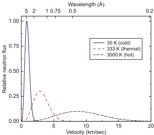 p10_0.jpg
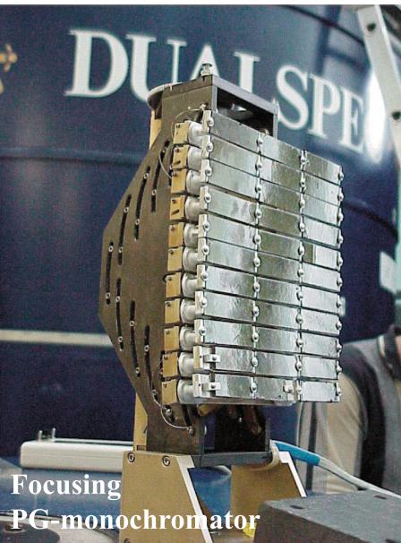 p11_0.jpg
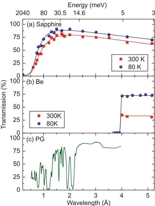 p11_1.jpg
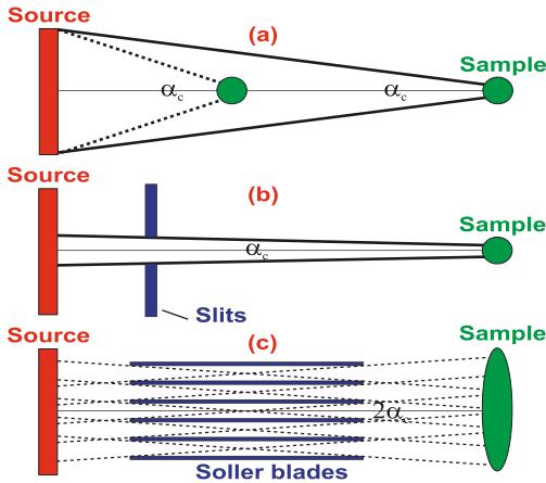 p13_0.jpg
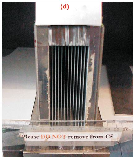 p13_1.jpg
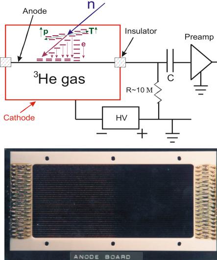 p14_0.jpg
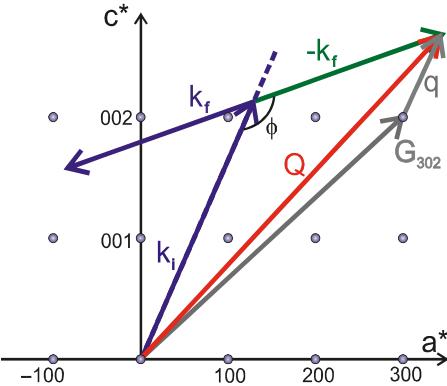 p15_0.jpg
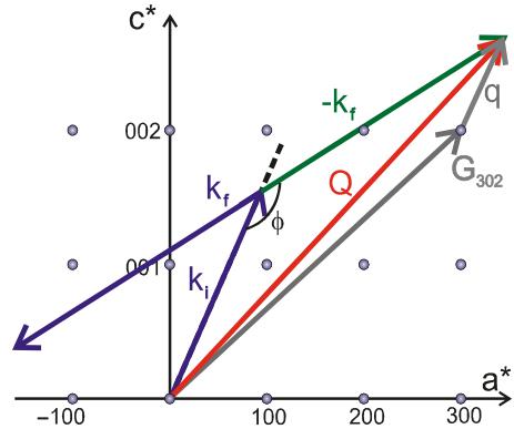 p15_1.jpg
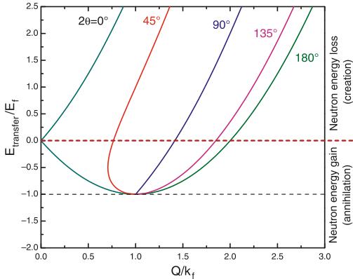 p15_2.jpg
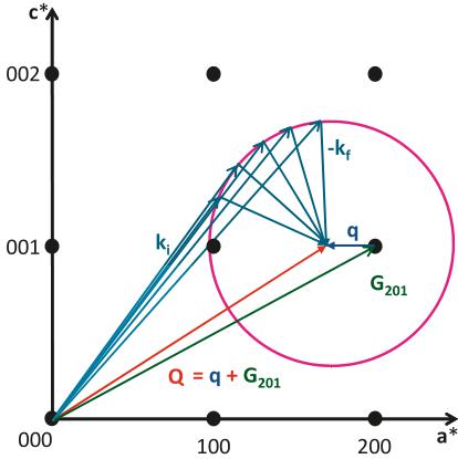 p16_0.jpg
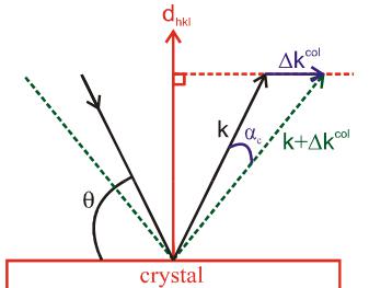 p17_0.jpg
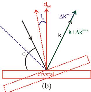 p17_1.jpg
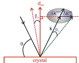 p17_2.jpg
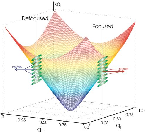 p17_3.jpg
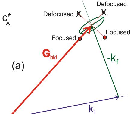 p18_0.jpg
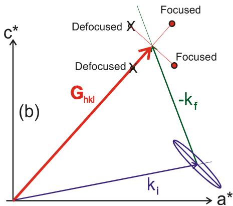 p18_1.jpg
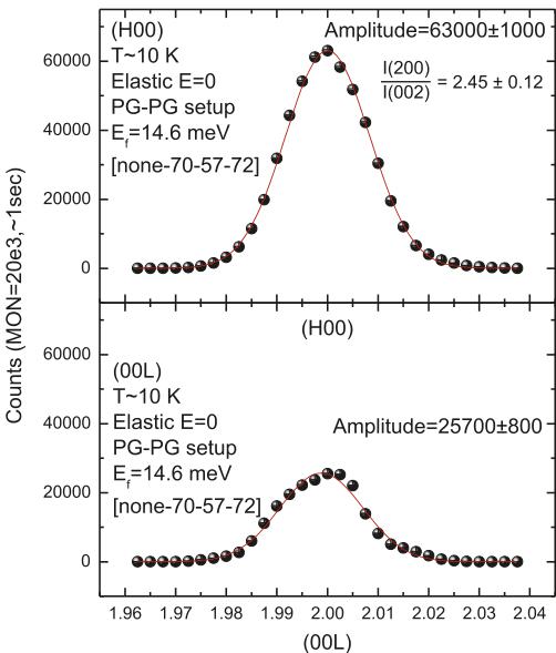 p19_0.jpg
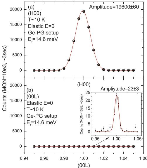 p19_1.jpg
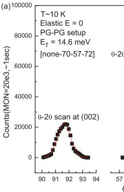 p20_0.jpg
 p20_1.jpg
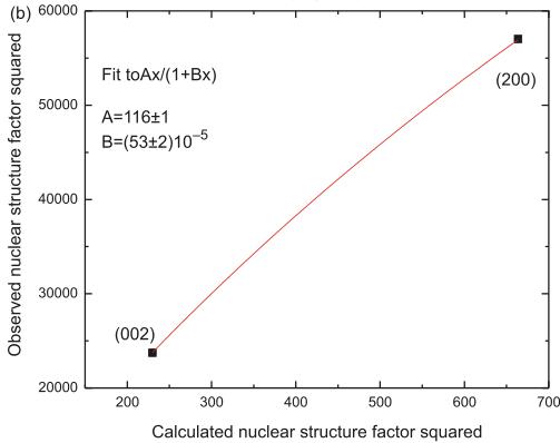 p20_2.jpg
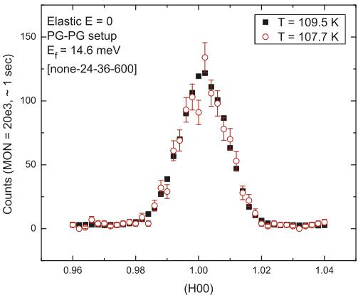 p20_3.jpg
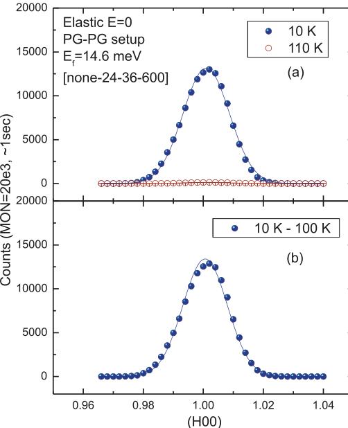 p21_0.jpg
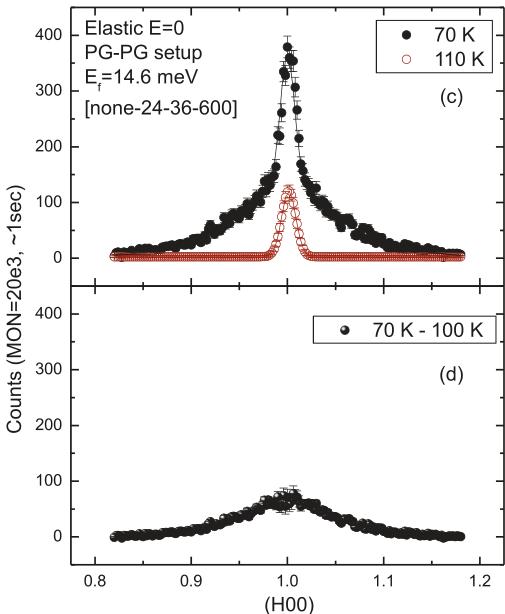 p21_1.jpg
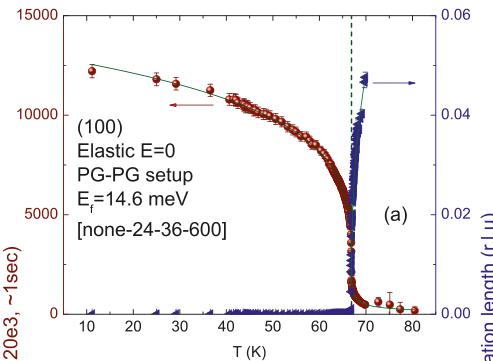 p22_0.jpg
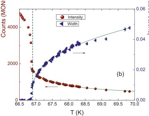 p22_1.jpg
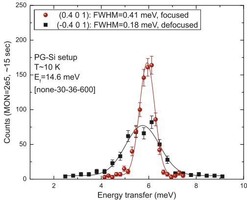 p22_2.jpg
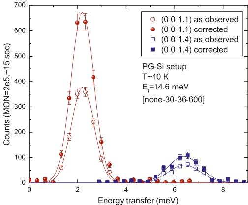 p22_3.jpg
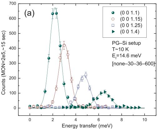 p23_0.jpg
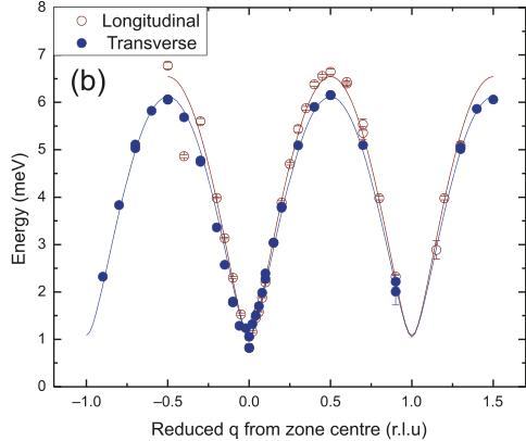 p23_1.jpg
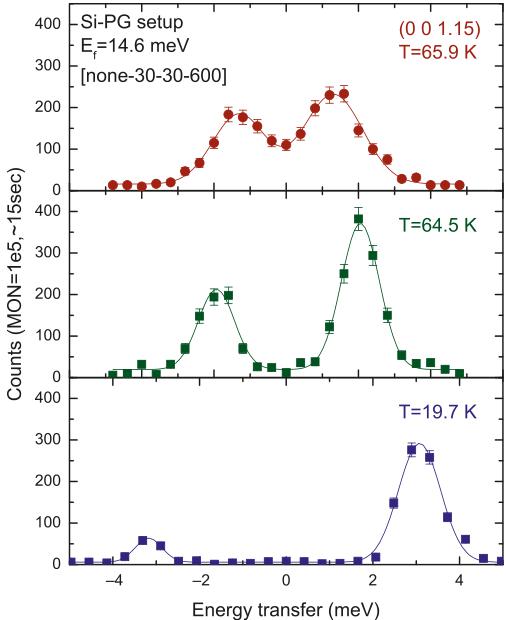 p23_2.jpg
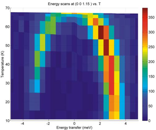 p24_0.jpg
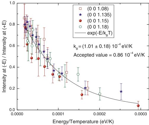 p24_1.jpg
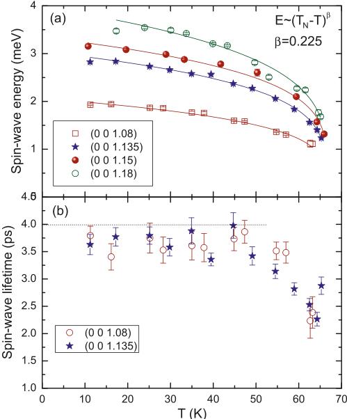 p25_0.jpg
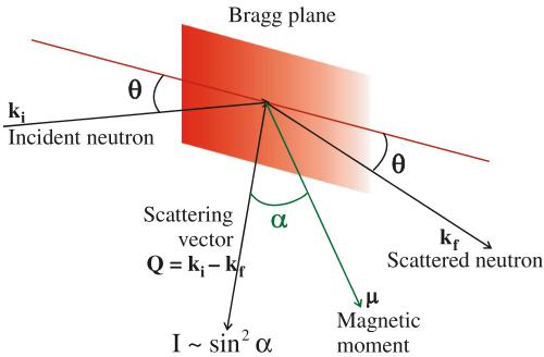 p2_0.jpg
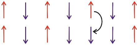 p3_0.jpg
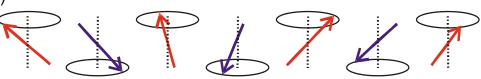 p3_1.jpg
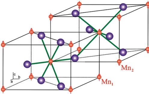 p4_0.jpg
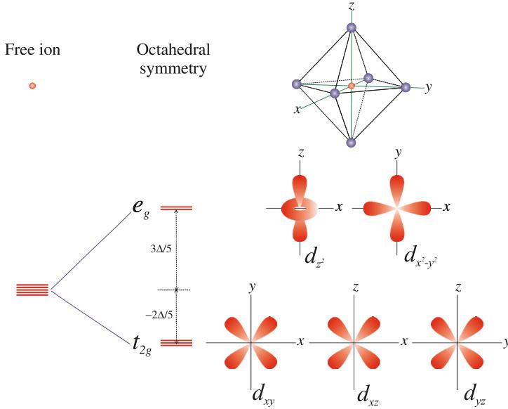 p5_0.jpg
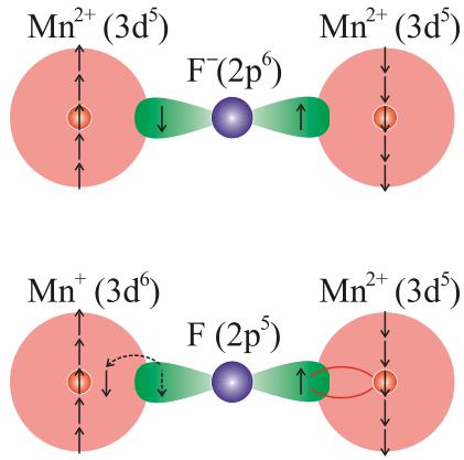 p6_0.jpg
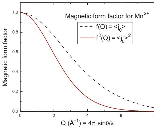 p8_0.jpg
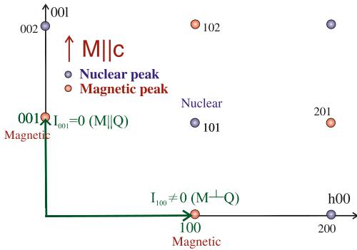 p8_1.jpg
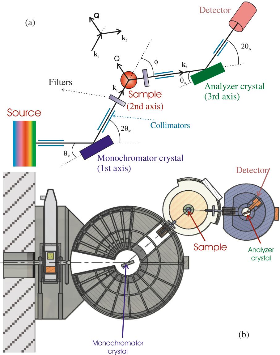 p9_0.jpg