| Experiment Temperature | 290 K |
|---|---|
| Parent Space Group | Fm-3m (#225) |
| Magnetic Space Group | Pn-3m' (#224.113) |
| Magnetic Point Group | m-3m' (32.4.121) |
| Lattice Parameters | 3.66800 3.66800 3.66800 90.00 90.00 90.00 |
|---|---|
| DOI | 10.1143/jpsj.21.1281 |
| Reference | H. Umebayashi and Y. Ishikawa, Journal of the Physical Society of Japan (1966) 21 1281-1294. |
Title
Antiferromagnetism of \( \gamma \) Fe-Mn Alloys
Authors
Hiromichi UMEBAYASHI \( ^{*} \) and Yoshikazu ISHIKAWA The Institute for Solid State Physics University of Tokyo, Tokyo
Materials Studied
- Disordered \( \gamma \) Fe-Mn alloys (polycrystalline and single crystal samples).
- Composition range: 20 to 50 at% Mn.
- Specific compositions studied (from Table I): 18.8 at% Mn, 20.1 at% Mn, 21.8 at% Mn, 25.9 at% Mn, 26.5 at% Mn, 28.1 at% Mn, 28.3 at% Mn, 30.9 at% Mn, 32.7 at% Mn, 37.0 at% Mn, 39.5 at% Mn, 43.4 at% Mn, 49.2 at% Mn.
- Starting materials: 99.9% pure electrolytic iron and 99.9% pure electrolytic manganese.
Key Information
- Crystal structure / space group:
- \( \gamma \) phase: f.c.c. (face-centered cubic)
- \( \varepsilon \) phase: h.c.p. (hexagonal close-packed, implied by martensitic transformation and x-ray peaks)
- \( \alpha \) phase: b.c.c. (body-centered cubic, trace in one sample)
- Magnetic structure: Generalized antiferromagnetic spin structure, intrinsically cubic. Spins on the four sublattices are directed toward the four different cube diagonals (\( \langle111\rangle \) directions), corresponding to an angle \( \theta = \cos^{-1}\sqrt{2/3} \).
- Magnetic ordering type and temperature:
- Antiferromagnetism.
- Néel temperature (T_N) range: 360 K (for 20.1 at% Mn) to 502 K (for 49.2 at% Mn). (Specific values for each composition are listed in Table I).
- T_N for pure \( \gamma \)-iron is estimated to be below \( 100^{\circ}K \).
- Propagation vector(s): Not explicitly stated as a vector, but magnetic peaks observed by neutron diffraction are (1 \( \overline{1} \) 0), (1 \( \overline{1} \) 2), and (2 \( \overline{2} \) 1), consistent with the proposed spin structure.
- Magnetic moments:
- Average atomic magnetic moment at \( 0^{\circ}K \): \( 1.7\mu_{B} \) (estimated by Kouvel and Kasper for 25 at% Mn).
- Average magnetic moment at room temperature: \( 1.5\pm0.1\mu_{B} \) (present study, for 30.9 at% Mn).
- Average magnetic moment at \( 0^{\circ}K \): \( 1.9\mu_{B} \) (extrapolated from present neutron diffraction data).
- Paramagnetic moment for 12 at% Mn-Fe alloy above T_N: approximately \( 0.5\mu_{B} \) (Nathans and Pickart).
- Lattice parameters:
- Lattice constant of the \( \gamma \) phase shows a break at about \( 150^{\circ} \) C.
- Estimated deviation of c/a ratio from unity is less than \( 10^{-3} \) (from Kouvel et al., consistent with cubic magnetic structure).
- Any other critical measured values:
- Susceptibility above T_N: approximately \( 1 \times 10^{-5} \) e.m.u./g.
- Maximum fractional anisotropy of susceptibility: 0.4%.
- Debye parameter: \( 0.35\AA^{2} \), corresponding to a Debye temperature of \( 425^{\circ}K \).
- Thermal expansion coefficient of \( \gamma \) phase (sample No. 7): \( 1.3 \times 10^{-3}/deg \) below T_N to \( 1.8 \times 10^{-5}/deg \) above T_N.
Synthesis Method
Poly-crystal samples: * Materials: 99.9% pure electrolytic iron and 99.9% pure electrolytic manganese. * Melting: Appropriate mixtures of the metals were melted several times in corundum crucibles in an induction furnace under argon at roughly one atmosphere pressure. * Heat Treatment (for susceptibility measurements): Ingots were shaped into rough cylinders (about 700 mg), sealed in fused silica tubes (about 7 mm in diameter and 45 mm in length) containing argon at approximately 15 mm Hg, and kept at \( 1040^{\circ} \) C for about 20 hours. * Composition Determination: Chemical composition of each sample was determined by colorimetric analysis on monitor alloys taken from the same ingots and subjected to the same heat treatments.
Single crystal samples: * Growth Method: Grown from the melt of a polycrystalline ingot by the Bridgman type method in an induction furnace under argon at roughly one atmosphere pressure. * Crucible Setup: A polycrystalline ingot was placed in a corundum crucible, which was then inserted into a graphite cylinder. These were placed in an outer corundum crucible. The ingot was heated indirectly by the graphite cylinder. * Temperature Profile: The graphite cylinder's shape and position were chosen to maximize the temperature gradient at the sample. The estimated maximum temperature was \( 1550^{\circ} \) C, maintained for about 30 minutes, then lowered at a rate of 3.2 cm/hour. * Post-growth Processing: The resulting specimen, containing several large grains, was etched in a saturated solution of \( FeCl_{3} \) and cut to yield several single crystals. * Annealing: Due to skeleton structure and diffuse Laue spots, the crystals were sealed in fused silica tubes under argon (15 mm Hg) and annealed at \( 1040^{\circ} \) C for 48 hours to sharpen Laue spots and largely eliminate the skeleton structure. * Orientation: Crystallographic orientations were determined by the Laue method. * Sample Preparation for Measurements: * For susceptibility: A rough parallelopiped (3.0 \( \times \) 3.0 \( \times \) 4.8 mm) with surfaces parallel to (100), (011), and (01 \( \overline{1} \) ). * For torque magnetometer: A disk (5.7 mm in diameter, 0.5 mm in thickness) with the main surface parallel to (100). * For neutron diffraction: Two cylindrical single crystals (3.00 mm and 2.35 mm diameters), both 6.30 mm in length parallel to [110].
Abstract
The antiferromagnetism of polycrystalline and single crystal samples of disordered \( \gamma \) Fe-Mn alloys containing between 20 to 50 at% Mn was investigated by means of a magnetic balance, a sensitive torque magnetometer and neutron diffraction. The alloys with 20 to 27 at% Mn exhibited \( \varepsilon\leftrightarrow\gamma \) transformation in the same temperature range as the magnetic transformation. The relation between the magnetic and the crystallographic transformations was investigated and a phase diagram of Fe-Mn alloys in this composition region was obtained. A neutron diffraction study of single crystal samples confirmed the generalized antiferromagnetic spin structure proposed by the powder neutron diffraction study of Kouvel and Kasper. The torque measurements, made on single crystals which had been cooled through the Néel point in a strong magnetic field, indicated that the spin structure is intrinsically cubic, the spins on the four sublattices being directed toward the different cube diagonals. The results are discussed from the viewpoint of a molecular field theory based on the localized electron model. However, the temperature dependence of the susceptibility below and above the Néel point cannot be interpreted on the basis of a localized electron model, although the latter can account for the proposed spin structure.
Main Content Summary
This paper presents a comprehensive investigation into the antiferromagnetism of disordered \( \gamma \) Fe-Mn alloys, covering a composition range of 20 to 50 at% Mn, using magnetic susceptibility, torque magnetometry, and neutron diffraction techniques on both polycrystalline and single crystal samples. The study first addresses the interplay between magnetic and crystallographic transformations in low manganese content alloys (20-27 at% Mn). It was found that these alloys undergo an \( \varepsilon\leftrightarrow\gamma \) martensitic transformation near the Néel temperature. Detailed X-ray diffraction and susceptibility measurements revealed that these two transformations are independent, with the magnetic transformation showing no thermal hysteresis, unlike the crystallographic one. A phase diagram for the \( \varepsilon\leftrightarrow\gamma \) transformation and the Néel temperature was established, showing that the \( \varepsilon \) phase is not ferromagnetic and has a lower susceptibility than the \( \gamma \) phase.
Magnetic susceptibility measurements on the single-phase \( \gamma \) alloys (28-49 at% Mn) showed an increase with temperature at low temperatures, a distinct break at the Néel temperature (T_N), and an almost temperature-independent behavior above T_N. The Néel temperatures ranged from 360 K to 502 K, increasing with Mn content. The temperature-independent susceptibility above T_N, which is quite large, and its similar composition dependence to the electronic specific heat coefficient, strongly suggest a dominant Pauli paramagnetism arising from collective electrons. Torque measurements on field-cooled single crystals indicated a very small magnetic anisotropy (maximum fractional anisotropy of 0.4%), implying an intrinsically cubic magnetic structure.
Neutron diffraction studies on single crystals confirmed the generalized antiferromagnetic spin structure previously proposed by Kouvel and Kasper from powder diffraction. The observation of specific magnetic peaks (e.g., (1 \( \overline{1} \) 0)) with long-range order and the absence of others, combined with the lack of significant magnetic anisotropy, led to the conclusion that the most probable spin structure is one with cubic symmetry where the four sublattice spins are directed along the four different \( \langle111\rangle \) body diagonals of the f.c.c. lattice. The average magnetic moment was determined to be \( 1.5\pm0.1\mu_{B} \) at room temperature, extrapolating to \( 1.9\mu_{B} \) at 0 K.
The paper discusses the proposed cubic spin structure in the context of nearest-neighbor exchange interactions and cubic anisotropy, showing it to be a stable configuration for identical spins. However, a significant contradiction arises when attempting to interpret the experimental susceptibility data using a localized electron model. Molecular field theory for the proposed cubic spin structure predicts a temperature-independent susceptibility below T_N and Curie-Weiss behavior above T_N, which is inconsistent with the observed monotonically decreasing susceptibility below T_N and nearly temperature-independent behavior above T_N. This discrepancy, coupled with the consistency of high-temperature susceptibility and electronic specific heat with a simple band model, strongly suggests that a collective electron model is a more appropriate framework for understanding the magnetic properties of these alloys.
Conclusion
The antiferromagnetism of Fe-Mn disordered alloys has been investigated by means of a magnetic balance, a sensitive torque magnetometer and a neutron diffractometer.
The alloys with 20~27 at% Mn exhibit an \( \varepsilon\leftrightarrow\gamma \) martensitic transformation in the temperature range around the Néel temperature of the \( \gamma \) phase. Measurements of the temperature dependence of the susceptibility and x-ray diffraction powder intensities revealed that the magnetic and crystallographic transformations are independent of each other. Thus the phase diagram of the \( \varepsilon\leftrightarrow\gamma \) transformation was deduced from susceptibility measurements.
The generalized antiferromagnetic spin structure of the \( \gamma \) Fe-Mn alloy proposed by Kouvel et al. was confirmed by the present single crystal neutron diffraction study. Though other possibilities were not completely eliminated, it was concluded that the most probable spin structure of the alloy is one with cubic symmetry in which the four different sublattice spins in the f.c.c. structure are directed along the four different body diagonals of the cubic lattice (see Fig. 13(iii)), as field cooling treatment in effective fields of up to 57.4 kOe did not produce any significant anisotropy in the susceptibility of the alloys.
Calculations showed that the cubic spin structure described above is one of the possible spin structures arising from nearest neighbor exchange interactions and cubic anisotropy in a f.c.c. lattice with identical spins. In reality, however, the Fe and Mn atoms are thought to have different magnetic moments, in which case local fluctuations of the spin direction are expected from the localized electron model, which does not seem to be in accordance with the observations.
The susceptibility of the \( \gamma \)-phase was confirmed to be almost temperature independent above \( T_{N} \). It was observed to decrease monotonically with decreasing temperature below \( T_{N} \) to liquid He temperature. The sharp rise of the susceptibility below \( 200^{\circ}K \) observed by Shiga and Nakamura \( ^{2)} \) was found to arise from impurities. On the basis of cubic spin structure described above, the temperature dependence of the susceptibility was calculated from the molecular field theory of localized spins. The result revealed that \( \chi \) should be temperature independent below \( T_{N} \). Above \( T_{N} \) \( \chi \) should of course follow the Curie-Weiss law. Thus below and above \( T_{N} \) experiment and theory were found to be in serious contradiction, indicating, therefore, that discussion of the spin structure in terms of a localized model is not valid in this alloy.
The composition dependence of the nearly constant susceptibility above \( T_{N} \) was found to be very similar to that of the electronic specific heat coefficient \( \gamma \) obtained by Gupta et al. \( ^{7)} \). The ratio of the susceptibility at \( 0^{\circ}K \) to \( \gamma \) and the tendency of the susceptibility to increase at high temperatures were found to be reasonably consistent with a simple band model. These facts suggest that the collective electron model is a better approximation in this alloy although a more rigorous approach is needed for further discussion. One of the interesting problems which remain to be investigated is to find if any difference in the magnetic behavior of Fe and Mn atoms in the Fe-Mn alloy can be detected. This will be a subject of a forthcoming paper.
Antiferromagnetism of \( \gamma \) Fe-Mn Alloys
Hiromichi UMEBAYASHI \( ^{*} \) and Yoshikazu ISHIKAWA
The Institute for Solid State Physics
University of Tokyo, Tokyo
(Received February 4, 1966)
The antiferromagnetism of polycrystalline and single crystal samples of disordered \( \gamma \) Fe-Mn alloys containing between 20 to 50 at% Mn was investigated by means of a magnetic balance, a sensitive torque magnetometer and neutron diffraction. The alloys with 20 to 27 at% Mn exhibited \( \varepsilon\leftrightarrow\gamma \) transformation in the same temperature range as the magnetic transformation. The relation between the magnetic and the crystallographic transformations was investigated and a phase diagram of Fe-Mn alloys in this composition region was obtained. A neutron diffraction study of single crystal samples confirmed the generalized antiferromagnetic spin structure proposed by the powder neutron diffraction study of Kouvel and Kasper. The torque measurements, made on single crystals which had been cooled through the Néel point in a strong magnetic field, indicated that the spin structure is intrinsically cubic, the spins on the four sublattices being directed toward the different cube diagonals. The results are discussed from the viewpoint of a molecular field theory based on the localized electron model. However, the temperature dependence of the susceptibility below and above the Néel point cannot be interpreted on the basis of a localized electron model, although the latter can account for the proposed spin structure.
§ 1. Introduction
The difference in the magnetic properties of \( \alpha \) -Fe (b.c.c.) and \( \gamma \) -Fe (f.c.c.) is very significant in understanding the magnetism of the 3d transition metals and alloys. In contrast with \( \alpha \) -Fe, the magnetic properties of \( \gamma \) -Fe have not yet been fully investigated because it is unstable at the low temperatures where any magnetic order takes place. In view of this situation, a detailed investigation of \( \gamma \) Fe-Mn alloys is very desirable, as at the solubility limit the \( \gamma \) phase in these alloys is richer in Fe than in any other magnetically ordered binary alloy of Fe.
The paramagnetic susceptibility behavior of polycrystalline specimens of several \( \gamma \) Fe-Mn alloys has been measured by Sedov \( ^{1)} \) and Shiga and Nakamura. \( ^{2)} \) They observed discontinuities in the susceptibility versus temperature curve ( \( \chi \) -T curve). One of the striking features of the \( \chi \) -T curves is that they are almost temperature independent at high temperatures. Kouvel and
Kasper \( ^{3)} \) carried out powder neutron diffraction measurements on an alloy with 25 at% Mn both above and below the temperature of the discontinuity in the \( \chi-T \) curve, and showed that below this point, the alloy became antiferromagnetic. The average atomic magnetic moment at \( 0^{\circ}K \) estimated from the coherent magnetic peaks was about \( 1.7\mu_{B} \) . Nathans and Pickart \( ^{4)} \) measured the paramagnetic neutron scattering from the 12 at% Mn-Fe alloy above the Néel point and obtained a much smaller moment of approximately \( 0.5\mu_{B} \) . These facts suggest that most of the localized moment which exists in the antiferromagnetic state is lost above the Néel temperature.
The present authors have made susceptibility measurements on polycrystalline specimens over a wide range of composition (18.2 at% to 49.2 at% Mn) and on single crystal specimens containing 30.9% Mn. The magnetic anisotropy of single crystals cooled through the Néel temperature has been measured in a magnetic field up to 57.4 kOe. The result of a preliminary neutron diffraction measurement on the single crystals at room temperature with and without an external magnetic field is also reported in the paper. The results are discussed in the light of the various existing models.
§ 2. Preparation of Alloys
(a) Poly-crystal
Poly-crystal Fe-Mn alloys were made from 99.9% pure electrolytic iron and 99.9% pure electrolytic manganese. Appropriate mixtures of the metals were melted several times in corundum crucibles in an induction furnace under argon at roughly one atmosphere pressure.
For susceptibility measurements the ingots were shaped into rough cylinders weighing about 700 mg. The latter were sealed in fused silica tubes about 7 mm in diameter and 45 mm in length containing argon at a pressure of approximately 15 mm Hg, and were kept at \( 1040^{\circ} \) C for about 20 hours. The susceptibility measurements at high temperature were carried out with these sealed samples, as the alloys are easily oxidized above \( 300^{\circ} \) C, even in a vacuum of \( 2 \times 10^{-5} \) mm Hg. For the measurements at low temperatures the samples were removed from the silica tubes.
The chemical composition of each sample was determined by colorimetric analysis on monitor alloys which were taken from the same ingots and underwent the same heat treatments as the samples.
(b) Single crystal
A single crystal of the Fe-Mn alloys was grown from the melt of a polycrystalline ingot by the Bridgman type method in an induction furnace under argon at roughly one atmosphere pressure. A polycrystalline ingot was put into a corundum crucible, which in turn was inserted into a graphite cylinder. These two were then placed in an outer corundum crucible. The ingot was thus heated indirectly by the graphite cylinder, whose shape and position relative to the inner corundum crucible were chosen so that the temperature gradient at the sample was as great as possible. The estimated maximum temperature of the sample was \( 1550^{\circ} \) C and it was kept for about 30 minutes at that temperature, and then lowered at the rate of 3.2 cm/hour. The resulting specimen, which contained several large grains, was etched in a saturated solution of \( FeCl_{3} \) and cut so as to give several single crystals of varying sizes. As these showed a rather noticeable skeleton structure and gave diffuse Laue spots, they were sealed in fused silica tubes under argon at 15 mm Hg and annealed at \( 1040^{\circ} \) for 48 hours. As a result of this the Laue spots became sharper and the skeleton structure largely, but not completely, disappeared. The crystallographic orientations of the single crystals were determined by the Laue method.
For susceptibility measurements a single crystal specimen was prepared in the shape of a rough parallelopiped with dimensions of \( 3.0 \times 3.0 \times 4.8 \) mm and with surfaces parallel to (100), (011) and (01 \( \overline{1} \) ) (No. 8a in Table I). For the torque magnetometer measurements a disk, 5.7 mm in diameter and 0.5 mm in the thickness, and with the main surface parallel to (100), was used (No. 8b).
Two cylindrical single crystals were made for the purpose of the neutron diffraction measurements with diameters of 3.00 mm (No. 8c) and 2.35 mm (No. 8a), both having a length of 6.30 mm parallel to [110]. The larger sample was also used for the torque magnetometer measurements.
All the samples used in this investigation are listed in Table I. The sample number, the manganese content, the crystal structures at room temperature, the type of sample and the measured Néel temperature of the \( \gamma \) -phase are also tabulated there.
§ 3. Experimental
(a) Susceptibility measurement
An automatic recording magnetic balance utilizing the Faraday method was used for the measurement of magnetic susceptibility. The pole faces of the electromagnet producing an inhomogeneous magnetic field were designed to give a constant field gradient in the vertical direction over a wide range of about \( \pm2.5 \) cm from the sample position, thus assuring excellent reproducibility of the data in different settings of the sample. The values of the field intensity H and field gradient dH/dz necessary for calculating the susceptibility were measured directly by a known small coil and a Cioffi type recording fluxmeter. The value of the saturation magnetization of a nickel sphere at room temperature measured by this balance agreed with the literature value to within 1%. The diamagnetic contributions of the sample holder and silica tubes were 10% of the total value at most and were subtracted by making a blank test.
Temperature of the sample was measured with a Pt-13% Rh in Pt thermocouple above room temperature and with a Cu-2% Co in Au thermocouple below.
The measurement of the temperature dependence of the susceptibility was mainly carried out at a fixed magnetic field. The temperature was varied continuously at rates of 1–3 degree/min. above room temperature and about 4 degree/min. below. At several fixed temperatures full magnetization-field curves were measured, particularly above room temperature.
(b) Anisotropy measurement
The anisotropy of the susceptibility in the single crystals was also measured by a sensitive automatic torque magnetometer originally designed for thin film measurements. The maximum torque which could be measured accurately by the torque meter was \( 1 \times 10^{-2} \) dyne cm.
The anisotropy was measured before and after the field cooling treatment which was carried out as follows. The samples were sealed in a silica tube, heated to about \( 250^{\circ} \) C (well above the Néel temperature \( 162^{\circ} \) C), and finally cooled to room temperature in 30 to 40 minutes in a magnetic field applied along the direction of one of the principal crystallographic axes. Two types of experiment were tried. In the first, the field cooling process was performed in a strong magnetic field applied either with a large electromagnet (45 kOe) or with a Bitter type solenoid magnet at the Central Laboratory of Hitachi Ltd. (90 kOe). The sample was then placed in the sensitive torque meter for anisotropy measurements. In the other sample was first placed in the torque meter and both the field cooling process (in a magnetic field of 15 kOe) and the measurement of the anisotropy were carried out in the same position.
The torque curves obtained were analyzed into Fourier components of \( \theta \) , \( 2\theta \) and \( 4\theta \) .
(c) Neutron diffraction measurement
A preliminary neutron diffraction study of the cylindrical single crystals No. 8c and No. 8d was carried out at room temperature with the neutron diffractometer of I.S.S.P. at the Japan Atomic Energy Research Institute. \( ^{5} \) The thermal neutron beam was monochromatized to a wave-length of \( 1.075\AA \) by the Bragg reflection from the (311) plane of lead.
§ 4. Experimental Results
(a) \( \gamma-\varepsilon \) transformation in low manganese alloys
An x-ray diffraction pattern of sample No. I showed peaks from both the \( \gamma \) and \( \varepsilon \) phases together with a trace of the \( \alpha \) phase. This alloy was found to be ferromagnetic at room temperature, and further investigation was therefore not attempted.
The other alloys were all paramagnetic and the magnetization curves were linear within experimental error at all temperatures up to a maximum field strength of 10 kOe.
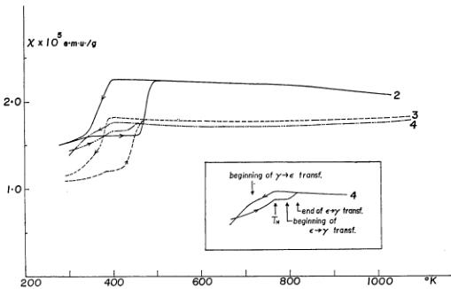
In the alloys No. 2 to No. 5, an x-ray examination revealed that the \( \gamma \) and \( \varepsilon \) phases coexist at room temperature. Their representative \( \chi-T \) curves above room temperature are shown in Fig. 1, in which the \( \chi-T \) curves can be seen to exhibit complicated behavior around \( 400^{\circ}K \) such as thermal hysteresis and discontinuities. The extent of thermal hysteresis was rather variable from cycle to cycle on heating and cooling, and accordingly the values of \( \chi \) at room temperature were different after each cycle. The temperatures where the breaks occur, however, were very reproducible. The amount of thermal hysteresis is thought to be sensitively dependent on the cooling rate of the sample. The thermal hysteresis itself is considered to arise from the reported matensitic transformation \( ^{6} \) between the \( \gamma \) and \( \varepsilon \) phases of the alloy. In order to find any possible correlation between this transformation and the magnetic transformation which is expected to occur in the same temperature range, detailed

Fig. 1. Magnetic susceptibility versus temperature of Fe-Mn alloys with 20 to 26 at % Mn. Numbers attached to curves indicate sample numbers as listed in Table I.
crystallographic and magnetic studies were carried out on samples No. 6 and No. 7, both of which have almost the same manganese content.
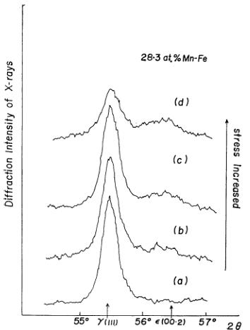
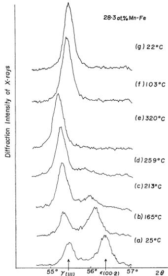
Although ordinary heat treatment gave a single \( \gamma \) phase, the \( \varepsilon \) phase appeared when the samples were stressed at room temperature. Figure 2 gives the changes in the main peaks of the x-ray diffraction pattern of the \( \gamma \) and \( \varepsilon \) phases when the surface of the sample was polished with emery paper. The two-phase state was also realized by cooling sample No. 7 from \( 800^{\circ} \) C under a shearing stress of about \( 10 \, g/cm^{2} \) . The temperature variation of the main peaks of both phases was studied

Fig. 2. Changes in x-ray diffraction patterns when the sample was polished with emery paper.
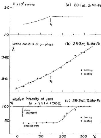
by means of a high temperature x-ray diffractometer and the results are shown in Fig. 3. The integrated intensities of the \( \gamma \) (111) peak relative to the total intensity of the peaks \( \gamma(111) \) and \( \varepsilon(00.2) \) and the lattice constant of the \( \gamma \) phase calculated from Fig. 3 are plotted as a function of temperature in Figs. 4(c) and (b) respectively. When heated, the \( \varepsilon \) phase begins to transform into the \( \gamma \) phase at about \( 170^{\circ} \) C and disappears.

Fig. 3. Temperature variation of x-ray diffraction patterns.
at about \( 270^{\circ} \) C. The \( \gamma \) phase is then stable even if it is cooled to room temperature. The lattice constant of the \( \gamma \) phase is found to have a break at about \( 150^{\circ} \) C. The temperature dependence of the magnetic susceptibility of sample No. 6 was measured in the stable \( \gamma \) phase during subsequent heating and cooling and is shown in Fig. 4(a).

Fig. 4. Temperature variations of a) susceptibility of \( \gamma \) phase of sample No. 6, b) lattice constant of \( \gamma \) phase, and c) relative intensity of \( \gamma(111) \) to \( \gamma(111) \) and \( \varepsilon(00.2) \) of sample No. 7, which was stress cooled from \( 800^{\circ} \) C.
The curve exhibits no thermal hysteresis and has a break at \( 147^{\circ} \) C similar to that reported at the antiferromagnetic Néel temperature. The temperature of the break is different from the temperatures at the beginning and the end of the \( \varepsilon\rightarrow\gamma \) transformation in Fig. 4(c) but coincides with the temperature of the break in Fig. 4(b). It is concluded therefore that there is no correlation between the magnetic and \( \varepsilon-\gamma \) crystallographic transformations in the alloy and that, although the latter transformation shows thermal hysteresis, the former, like most magnetic transformations, does not.
In the light of the above results, the \( \gamma \) -T curves in Fig. 1 can be explained in the way illustrated for sample No. 4 in the inset to Fig. 1. The break corresponding to the Néel temperature appears at the same temperature on heating and cooling. In the heating curve there are two more breaks corresponding to the beginning and the end of the \( \varepsilon\rightarrow\gamma \) transformation. In the cooling curve there is one more break which corresponds to the beginning of the \( \gamma\rightarrow\varepsilon \) transformation. The end of the \( \gamma\rightarrow\varepsilon \) transformation cannot be attained even below room temperature so that the two-phase state is realized at room temperature.
The temperatures of the \( \varepsilon\rightarrow\gamma \) transformation determined in this way are plotted as a function of manganese composition in Fig. 5 together with the previous results summarized in Hansen. \( ^{6} \) The results obtained for No. 7 (28.3 at%) are connected by dotted lines, because the \( \varepsilon \) phase of No. 7 was realized by stress cooling. The transformation temperatures of this sample are not necessary the same as those of the normal \( \varepsilon \) phase. The Néel temperature determined in the present study are also shown in the figure.

Fig. 5. Phase diagram of Fe-Mn alloys.
beginning of \( \varepsilon\rightarrow\gamma \) transformation - - - authors', --- Hansen's end of \( \varepsilon\rightarrow\gamma \) transformation - - - authors', --- Hansen's ☐ and ▲ are respectively beginning and end of \( \varepsilon\rightarrow\gamma \) transformation of \( \varepsilon \) phase realized by stress cooling beginning of \( \gamma\rightarrow\varepsilon \) transformation
Néel temperature - - - - - - - - - - - - - - - - - - - -
The above experiments also show that the \( \varepsilon \) phase of Fe-Mn alloys is not ferromagnetic and has a susceptibility smaller than that of the \( \gamma \) phase and that the thermal expansion coefficient of the alloy in the \( \gamma \) phase changes discontinuously at \( T_{N} \) , for example from \( 1.3 \times 10^{-3}/deg \) below \( T_{N} \) \( T_{N} \) to \( 1.8 \times 10^{-5}/deg \) above \( T_{N} \) in sample No. 7. (b) Susceptibility in \( \gamma \) phase
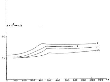
Samples No. 6 to No. 13 are single phase with the \( \gamma \) structure in the temperature range \( 77^{\circ}K \) to \( 1050^{\circ}K \) . The representative \( \chi-T \) curves are shown in Fig. 6. For sample No. 6 the measure-
ment was extended to liquid He temperature. The susceptibility increases with increase of temperature at low temperatures, shows a break at \( T_{N} \) and becomes almost temperature independent above \( T_{N} \) , with a slight tendency to increase at higher temperatures.

Fig. 6. Magnetic susceptibility versus temperature of Fe-Mn alloys with the f.c.c. structure.
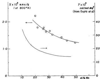
From the figure, it can be seen that the susceptibility above \( T_{N} \) does not follow the Curie-Weiss law, so that the main contribution is probably the Pauli paramagnetism of collective electrons. The value of \( \chi \) above \( T_{N} \) is approximately \( 1 \times 10^{-5} \) e.m.u./g, which is very large for Pauli paramagnetism, even larger than the known maximum value of \( 7.5 \times 10^{-5} \) e.m.u./g for Pd. The values of \( \chi \) for the various samples at \( 800^{\circ} \) K in the roughly constant susceptibility region above \( T_{N} \) are plotted as a function of manganese content in Fig. 7, where the composition dependence of the electronic specific heat coefficient \( \gamma^{*} \) of the same alloys obtained by Gupta et al. \( ^{[7]} \) is also shown. The figure indicates that the composition dependences of \( \chi \) and \( \gamma \) are very similar to each other, which favors the hypothesis that the susceptibility arises mainly from the collective electrons. The behavior of the susceptibility below \( T_{N} \) is more or less similar to that of the usual ionic antiferromagnets where the localized electron model is valid. \( ^{[8]} \) However, we shall show in a later section that this behavior

Fig. 7. Composition dependence of magnetic susceptibilities at \( 800^{\circ} \) K and comparison with electronic specific heats obtained by Gupta et al. \( ^{[7]} \)
Table I. Fe-Mn alloys used in this investigation.
| Sample No. | at% Mn | Phase at 25°C | Type | T_{N} of γ-phase (°K) |
| 1 | 18.8 | α, γ, ε | poly | |
| 2 | 20.1 | γ, ε | poly | 360 |
| 3 | 21.8 | γ, ε | poly | 390 |
| 4 | 25.9 | γ, ε | poly | 401 |
| 5 | 26.5 | γ, ε | poly | 403 |
| 6 | 28.1 | γ | poly | 420 |
| 7 | 28.3 | γ(ε) | poly | 421 |
| 8a | single (parallelepiped) | 435 | ||
| 8b | 30.9 | γ | single (disk) | |
| 8c | single (cylinder) | |||
| 8d | single (cylinder) | |||
| 9 | 32.7 | γ | poly | 450 |
| 10 | 37.0 | γ | poly | 458 |
| 11 | 39.5 | γ | poly | 465 |
| 12 | 43.4 | γ | poly | 485 |
| 13 | 49.2 | γ | poly | 502 |
- Stable in the stressed state.
cannot in fact be interpreted on the basis of a localized electron model.
Shiga and Nakamura \( ^{a)} \) have reported a rather sharp rise in \( \chi \) at low temperatures for alloys containing 35 to 55 at% Mn. This phenomenon could not be observed in the present study. A measurement was carried out by the present authors on samples taken from the same ingot used by Shiga and Nakamura in order to check this disagreement. The results revealed that the phenomenon was not intrinsic to Fe-Mn alloys but was due to materials stuck to the inside walls of the silica tubes containing the samples.
The Néel temperatures of the Fe-Mn alloys determined from the \( \chi-T \) curves are listed in Table I and are plotted as a function of manganese content in Fig. 5. In the alloys with 30 to 50 at% Mn, the values of \( T_{N} \) are in good agreement with those of Sedov \( ^{1)} \) and Shiga and Nakamura \( ^{2)} \) but in the alloys with a smaller manganese content, the values are considerably larger than those of Sedov, the difference amounting to 70°K for the alloy with 20 at% manganese.
Although extrapolation of the \( T_{N} \) curve to the point corresponding to pure \( \gamma \) -iron cannot be made with accuracy, at least it can be said that \( T_{N} \) for \( \gamma \) -iron is below \( 100^{\circ}K \) , which does not conflict with the reports of other investigators. \( ^{9,10} \)
(c) Anisotropy of the susceptibility
The anisotropy of the susceptibility was measured on the single crystal samples No. 8a to No. 8c. For sample No. 8a, \( \chi-T \) curves were measured in the [100] and [011] directions. The curves coincided with each other within experimental error and the shapes of the curves were quite similar to those of polycrystalline samples. No anisotropy was detected either when the magnet was rotated about a vertical axis corresponding to rotation of the applied field within the (100) and (011) planes.
Similar measurements in the (100) plane were also made after the specimen was cooled through the Néel temperature with an applied magnetic field to 49 kOe in the [010] direction, but no change was observed however.
More sensitive measurements of the anisotropy were performed with the torque magnetometer. The measured torque was found to be very sensitive to the position of the specimen, so that the reproducibility of the measurements was not particularly good. This is because the force acting on the specimen due to small inhomogeneities in the magnetic field produces an apparent torque of the same order of magnitude as that of the expected anisotropy. In spite of this difficulty, however, an estimate of the order of magnitude of the maximum anisotropy of the specimen could be made.
The torque curves obtained consist mainly of a \( 2\theta \) Fourier component. A smaller but appreciable amount of the \( \theta \) component and a negligible amount of the \( 4\theta \) component were also found. The magnitude of the \( 2\theta \) component for each sample in a magnetic field of 4.9 kOe is summarized in Table II. It is noted that in the case of sample No. 8a, which is in the shape of a parallelepiped, the shape anisotropy gives a torque of the same order of magnitude as the observed one. In the case of sample No. 8c, the direction of the field applied in the cooling process was not along a principal axis so that the effective field strength was only 57.4 kOe.
As can be seen in the table, the \( 2\theta \) components of the torque \( \left|L_{2\theta}\right| \) have similar orders of magnitude regardless of the strength and the direction of the field cooling and of the weight of the sample. The value is about \( 5\times10^{-1} \) dyne·cm/g at the greatest.
The torque per gram L caused by the anisotropy of the susceptibility \( \chi(\mathrm{e.m.u./g}) \) in the measured plane is expressed as follows:
\[ L{=}\frac{H^{2}}{2}\frac{\partial\chi}{\partial\theta}, \quad (1) \]
where H is the measuring field and \( \theta \) is the angle
Table II. Results of torque measurement at 4.9 kOe.
| Sample No. | Weight (g) | Measured Plane | Field Direction | Colling Field (kOe) | 2θ component (dyne·cm.) | 2θ component (dyne·cm/g) |
| No. 8a | 0.296 | (100) | 5.6×10⁻² | 1.9×10⁻¹ | ||
| (100) | [010] | 15 | 5.6×10⁻² | 1.9×10⁻¹ | ||
| (011) | [100] | 49 | 4.4×10⁻² | 1.5×10⁻¹ | ||
| No. 8b | 0.094 | (100) | 3.5×10⁻² | 3.7×10⁻¹ | ||
| (100) | [010] | 15. | 3.8×10⁻² | 4.0×10⁻¹ | ||
| No. 8c | 0.321 | (110) | [110] | 81 | 3.1×10⁻² | 1.0×10⁻¹ |
between H and a fixed reference direction in the measured plane of the crystal. As will be seen later, neutron diffraction reveals that Fe-Mn alloys are magnetically tetragonal (or cubic in a special case). Therefore the susceptibility can be expressed by two components \( \chi_{e} \) , (the susceptibility parallel to the tetragonal c axis) and \( \chi_{a} \) (the susceptibility perpendicular to the c axis). Furthermore, single crystal sample are generally considered to have many antiferromagnetic domains with tetragonal axis parallel to the different cubic axes. If we write the volume fractions of the x, y and z domains (domains with the tetragonal c axis parallel to cubic [100], [010] and [001] axes respectively) as \( v_{x} \) , \( v_{y} \) , and \( v_{z} \) respectively, the net susceptibilities in the (100) and (110) planes are expressed as follows:
\[ \chi(\theta)_{(100)}=v_{x}\chi_{a}+v_{z}\chi_{a}+v_{y}\chi_{e}+\Delta v\Delta\chi\cos^{2}\theta, \quad (2a) \]
with
\[ \Delta v=v_{y}-v_{z}\mathrm{a n d}\Delta\chi=\chi_{a}-\chi_{e}, \quad (2b) \]
and
\[ \chi(\theta)_{(110)}=\frac{1}{2}(\chi_{a}+\chi_{e}+v_{z}\Delta\chi)+\Delta v\Delta\chi\cos^{2}\theta, \quad (3a) \]
with
\[ \Delta v=\frac{1}{2}\left(v_{x}+v_{y}\right)-v_{z}. \quad (3b) \]
In both equations the angle \(\theta\) is measured with reference to the [001] axis. From eqs. (1), (2a), and (3a), the torque \(L_{2\theta}\) is given by
\[ L_{2\theta}=\frac{1}{2}H^{2}\Delta v\Delta\chi\cdot\sin2\theta. \quad (4) \]
Then the fractional anisotropy of the susceptibility is calculated from the equation
\[ \frac{\Delta v\Delta\chi}{\chi}=\frac{2\left|L_{2\theta}\right|_{\max}}{H^{2}\chi}. \quad (5) \]
The maximum fractional anisotropy estimated using eq. (5) and substituting the greatest observed value obtained for the torque is only 0.4%, which suggests that the sample has practically no anisotropy. Since this value is affected very little by the field cooling treatment up to an effective field of 57.4 kOe, it seems most likely that \( \Delta\chi \) and not \( \Delta v \) is responsible for the smallness of the observed effect.
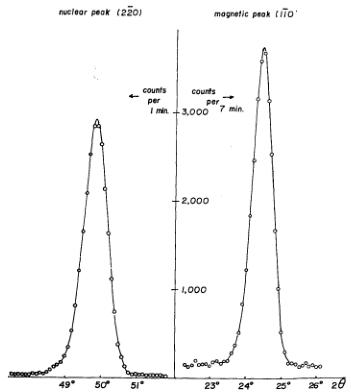
(d) Neutron diffraction
In the present experiment, six nuclear peaks (1 \( \overline{1} \) 1, 002, 220, 1 \( \overline{1} \) 3, 222 and 004), three magnetic peaks (1 \( \overline{1} \) 0, 1 \( \overline{1} \) 2, and 2 \( \overline{2} \) 1), and two “forbidden” peaks ( \( \frac{1}{2} \) \( \frac{1}{2} \) 0) and (001) from samples No. 8c and No. 8d were examined. Typical examples of both nuclear and magnetic peaks are shown in Fig. 8. It should be noted that the half width of the magnetic peak (1 \( \overline{1} \) 0) is almost the same as that of the nuclear peak (2 \( \overline{2} \) 0), indicating that proper long-range magnetic order is established in the sample. The observed integrated intensities are listed in Table III. The integrated nuclear and magnetic intensities \( I_{N}(hkl) \) and \( I_{M}(hkl) \) are expressed as follows:
\[ I_{N}=\frac{A v}{\sin2\theta_{B}}\exp\left(-2B\frac{\sin^{2}\theta_{B}}{\lambda^{2}}\right)\times\left\{\sum_{1=i}^{4}\bar{b}\exp2\pi i(h x_{i}+k y_{i}+l z_{i})\right\}^{2}, \]

Fig. 8. Neutron diffraction patterns of nuclear peak (220) and magnetic peak (110).
Table III. Integrated intensities of neutron diffraction. Contribution from \( \lambda/2 \) contamination have been subtracted.
| Peak | Kind of Peak \( ^{(a)} \) | I (counts/min) | |
| No. 8c | No. 8d | ||
| \( \frac{3}{2} \) 0 | 0 > 50 | ||
| 0 0 1 | 0 < 50 | ||
| 1 1 0 | M | 3,562 | 2,685 |
| 1 1 1 | N | 38,512 | 26,815 |
| 1 1 1 | N | 39,478 | |
| 0 0 2 | N | 34,729 | 21,590 |
| 1 1 2 | M | 134 | 114 |
| 1 1 2 | M | 209 | |
| 2 2 0 | N | 24,084 | 15,393 |
| 2 2 1 | M | 144 | |
| 2 2 1 | M | 133 | |
| 1 1 3 | N | 18,249 | |
| 2 2 2 | N | 17,594 | 15,900 |
| 0 0 4 | N | 13,811 | 10,463 |
(a) N: nuclear peak
M: magnetic peak
and
\[ \begin{array}{r}{I_{M}=\frac{A v}{\sin2\theta_{B}}\exp\left(-2B\frac{\sin^{2}\theta_{B}}{\lambda^{2}}\right)\left(\frac{e^{2\gamma_{r}}}{m c^{2}}\right)^{2}}\\ {\times\bar{S}^{2}\bar{f}^{2}[F]^{2},}\end{array} \quad (7) \]
with
\[ F=\sum_{i=1}^{4}\{\alpha_{i}-n(\alpha_{i}n)\exp2\pi i(h x_{i}+k y_{i}+l z_{i}), \quad (8) \]
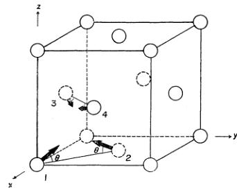
where \( \alpha_{i} \) , n, v and A are respectively a unit vector parallel to the i-th spin in Fig. 9, a unit vector normal to the reflection plane, the volume of the sample and a scale factor. All other symbols have the conventional meanings. For a spin structure with the magnetic tetragonal axis parallel to the cubic [001] as described in Fig. 9, the magnetic structurs factor F in eq. (8) is calculated in a straightforward way to be

Fig. 9. Spin configuration compatible with neutron diffraction results.
\[ \begin{aligned}|F|^{2}=&16\left(1-\frac{l^{2}}{s^{2}}\right)\sin^{2}\theta,\quad&for h,k;even l;odd\\&h,k;odd,l;even\\&for h,l;even k;odd\\|F|^{2}=&8\left(1-\frac{k^{2}}{s^{2}}\right)\cos^{2}\theta,\quad&h,l;odd,k;even\\&(or interchange\\&between h and k)\end{aligned} \]
\[ |F|^{2}=0,\quad\text{for other }h,k,l\text{ combinations with} \]
\[ s=\sqrt{h^{2}+k^{2}+l^{2}}, \quad (9) \]
where \(\theta\) is defined as illustrated in Fig. 9.
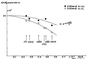
The angular dependence of the integrated intensities of the nuclear peaks per unit volume of the sample is shown in Fig. 10. As is seen in the figure, the curve for No. 8c falls anomalously rapidly, though the other curve has a normal form. The situation was not improved when the slit in front of the \( BF_{3} \) counter was replaced by a wider one. Possible secondary extinction effects would reduce the intensities of low angle peaks most severely and thus cannot explain the experimental observations. Both curve can be extrapolated to approximately the same value at \( \theta_{B}=0 \) , however, and the reason for their different angular dependence is not known. In the present study, the integrated intensities (both nuclear and magnetic) of sample No. 8c were scaled to those of sample No. 8d as far as possible.

Fig. 10. Angular dependence of integrated intensities of nuclear peaks per unit volume multiplied by \( \sin 2\theta_{B} \) for both samples No. 8c and No. 8d.
The Debye parameter determined from the angular dependence of the nuclear peaks is about \( 0.35\AA^{2} \) , which corresponds to a Debye temperature of \( 425^{\circ}K \) . This value agrees fairly well with value \( 405^{\circ}K \) obtained by Gupta et al. \( ^{7)} \) for an alloy with the composition \( 30.9\ at\% \) Mn-2.5 at% C-66.6 at% Fe.
All the magnetic peaks expected from the spin structure of Fig. 9 were observed with the proper intensity ratios and neither \( \left(\frac{1}{2}\frac{1}{2}0\right) \) nor (001) was observed. The absence of any satellite peaks was also confirmed.
The angle \( \theta \) could not be determined in the present study because of the lack of knowledge about the antiferromagnetic domain distribution. If the distribution of domains with magnetic tetragonal axes parallel to the cubic [100], [010] and [001] axes is defined as before as \( v_{x} \) , \( v_{y} \) , and \( v_{z} \) respectively, the average structure factors of the main magnetic peaks are calculated easily using eq. (9).
\[ \begin{aligned}&|F_{av1}\overline{1}0|^{2}=16\left(v_{z}\sin^{2}\theta+\frac{v_{x}+v_{z}}{2}\cos^{2}\theta\right)\\&|F_{av1}\overline{1}2|^{2}=\frac{16}{3}\left(v_{z}\sin^{2}\theta+\frac{v_{x}+v_{y}}{2}\cos^{2}\theta\right)\\&|F_{av2}\overline{2}1|^{2}=\frac{128}{9}\left(v_{z}\sin^{2}\theta+\frac{v_{x}+v_{v}}{2}\cos^{2}\theta\right)\\ \end{aligned} \quad (10) \]
As is apparent in eq. (10), there is a common factor containing the volume fractions \( v_{x} \) , \( v_{y} \) , \( v_{z} \)
and the spin direction \( \theta \) in the intensity expression, and it is therefore not possible to determine these quantities from the neutron diffraction study.
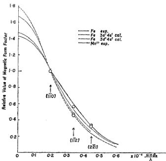
On the other hand, the magnetic form factor \( \bar{f} \) in eq. (7) can be deduced irrespective of the domain distribution of the sample by virtue of the same reasoning. A preliminary magnetic form factor calculated in this way is shown in Fig. 11 together with some available theoretical and experimental form factors of Fe and Mn. In the figure, the form factor is normalized to the value of \( (1\bar{1}0) \) for convenience. With the calculated form factor of the Fe \( 3d^{6}4s^{2} \) configuration, which seems to give the best fit to the experimental points, the average magnetic moment was found to be about \( 1.5\pm0.1\mu_{B} \) at room temperature. The temperature variation of the average moment determined by neutron diffraction suggests that the moment at \( 0^{\circ}K \) is \( 1.9\mu_{B} \) .

Fig. 11. Magnetic form factor reduced by the value of \( (1\bar{1}0) \) and comparison with available magnetic form factors relating to Fe and Mn.
The effect of an applied field on the crystal was checked by neutron diffraction on sample No. 8c at room temperature. This experiment is important in the interpretation of the results of magnetic anisotropy measurements because any change in domain distribution caused by the magnetic field used to make the measurement must be taken into account. No change in intensity of the \( (1\bar{1}0) \) reflection was observed when the field of 13 kOe was applied in the \( [1\bar{1}0] \) direction.
§ 5. Discussion
(a) Spin structure
The neutron diffraction study of single crystal samples is in agreement with the generalized spin structure proposed by Kouvel et al. \( ^{3} \) although \( \theta \) cannot be determined. The field cooling experiment described in § 4c strongly suggests that the anisotropy of the susceptibility is very small indicating that the crystal is magnetically cubic. The only cubic structure compatible with the neutron diffraction results is that in which \( \theta = \cos^{-1}\sqrt{2/3} \) such that each of the spins is directed along a different \( \langle111\rangle \) direction. This conclusion is also consistent with the x-ray results by Kouvel et al. \( ^{3} \) namely that the estimated deviation of the c/a ratio from unity is less than \( 10^{-3} \) .
This cubic spin structure can be shown to be one of this possible spin structures expected from consideration of nearest neighbor exchange interactions between the localized moments and the cubic anisotropy in the f.c.c. lattice as follows.
First we discuss the general spin configuration obtained by minimizing the nearest neighbor exchange energy, assuming that the magnitudes of the four spins located on different sublattices are identically S. If the directional cosines of a spin on the i-th sublattice are \( \alpha_{iz} \) , \( \alpha_{ix} \) , and \( \alpha_{iz} \) , the exchange energy density of the system is
\[ E_{e z}=-2J\sum_{i>j}\mathbf{S}_{i}\mathbf{S}_{j}=-2N J S^{2}\sum_{\langle i j\rangle}\alpha_{i}\alpha_{j}, \quad (11) \]
where J and N are the exchange integral and the number of atoms per unit volume respectively. \( \sum_{i} \) is the summation over the six nearest neighbor pairs in Fig. 9. The minimization of the energy \( E_{ex} \) under the condition
\[ \alpha_{i x}^{2}+\alpha_{i y}^{2}+\alpha_{i z}^{2}=1, \quad (12) \]
can be carried out by the method of Lagrangian multipliers as shown in the Appendix. The results of the calculation are illustrated in Fig. 12 and the angles between spins in this configu-

Fig. 12. Spin configuration minimizing the nearest neighbor exchange interactions in f.c.c. lattice with identical spins.
Table IV. Angles between spins.
| \( S_{1} \) | \( S_{2} \) | \( S_{3} \) | \( S_{4} \) | |
| \( S_{1} \) | 0 | \( \varphi \) | \( \varphi \) | \( \varphi' \) |
| \( S_{2} \) | \( \varphi \) | 0 | \( \varphi' \) | \( \varphi \) |
| \( S_{3} \) | \( \varphi \) | \( \varphi' \) | 0 | \( \varphi \) |
| \( S_{4} \) | \( \varphi' \) | \( \varphi \) | \( \varphi \) | 0 |
ration are tabulated in Table IV.
The following condition is imposed upon the three angles \(\varphi\), \(\varphi'\) and \(\varphi''\) in the table.
\[ \cos\varphi+\cos\varphi+\cos\varphi^{\prime}=-1. \quad (13) \]
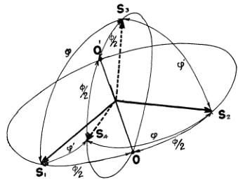
The results can be understood as follows. Consider two spin pairs, say \( (S_{1}, S_{2}) \) and \( (S_{3}, S_{4}) \) , with an intra pair angle \( \varphi \) and with their bisector common (segment OO' in Fig. 12). Then those pairs have freedom of rotation around the bisector so long as the angles \( \varphi \) and \( \varphi' \) determining the inter pair angles satisfy the condition (13). Thus, as far as the exchange interaction between nearest neighbors is concerned, two degrees of freedom are left unknown.
Next we consider the effect of the cubic anisotropy energy density up to terms of the sixth order.
\[ \begin{aligned}E_{an}=&K_{1}\sum_{i=1}^{4}\left(\alpha_{ix}^{2}\alpha_{iy}^{2}+\alpha_{iy}^{2}\alpha_{ix}^{2}+\alpha_{iz}^{2}\alpha_{ix}^{2}\right)\\&+K_{2}\sum_{i=1}^{4}\alpha_{ix}^{2}\alpha_{iy}^{2}\alpha_{ix}^{2}.\end{aligned} \quad (14) \]
The condition minimizing this energy can be found in standard texts \( ^{12} \) and is tabulated in the left part of Table V. The stable spin configura-
Table V. Easy Directions and Inter-spin Angles.
| Case No. | \( K_{1} \) | \( K_{1} \) | Easy direction | Inter-spin angles | |||
| \( \varphi \) | \( \varphi' \) | \( \varphi'' \) | |||||
| 1 | \( K_{1}>0 \) | \( K_{1}>-\frac{1}{9}K_{2} \) | <100> | 0 | 180° | 180° | |
| 2 | \( K_{1}<0 \) | \( K_{1}>-\frac{4}{9}K_{2} \) | <110> | 180° | 90° | 90° | |
| 3 | \( K_{1}<-\frac{1}{9}K_{2} \) | \( K_{1}<-\frac{4}{9}K_{2} \) | <111> | \( \cos^{-1}\frac{1}{\sqrt{3}} \) | \( \cos^{-1}\frac{1}{\sqrt{3}} \) | <cos^{-1}\frac{1}{\sqrt{3}} | |
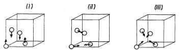
tions are determined so as to minimize the total energy \( E_{ex} + E_{an} \) . It can easily be found that the inter-spin angles listed in the right part of Table V minimize both \( E_{ex} \) and \( E_{an} \) . Therefore the spin configurations corresponding to these inter-spin angles, which are illustrated in Fig. 13, are the stable configurations of the system. The spin configuration in the third case (Fig. 13 iii), which has cubic symmetry, in the one believed to be realized in Fe-Mn alloys in the present study.

Fig. 13. Stable spin structures which minimize exchange interaction energy and anisotropy energy of the f.c.c. structure with identical spins.
It is to be noted, however, that quite different magnetic moments may reside on Fe and Mn atoms, since the internal field acting on the \( Fe^{57} \) nuclei (30~50 kOe) in the alloy is reported to be much smaller than that expected from the average moment obtained by neutron diffraction. \( ^{[11,13]} \) The effect of a random distribution of different magnetic moments on the spin configuration is very complicated, but it can safely be said that the directions of the spins may be distributed over a small angle around the \( \langle111\rangle \) direction by local inhomogeneities in the magnetic interaction and the anisotropy if we adopt a localized model. Such a distribution would broaden the magnetic diffraction peaks in comparison with the nuclear peaks in contradiction to the experimental observations. Thus, it appears that the spin structure of this alloy cannot be simply interpreted by consideration of nearest neighbor interactions and anisotropy based on a localized electron model.
(b) Susceptibility
The temperature dependence of the magnetic susceptibility below \( T_{N} \) was found to be similar to that usually displayed by ionic antiferromagnets. However, in the case of the non-collinear and isotropic spin structure shown in Fig. 13(iii), the concept of parallel and perpendicular susceptibilities, \( \chi_{\parallel} \) and \( \chi_{\perp} \) can no longer be adopted and the temperature dependence of this suscepti-
bility is not evident even if the discussion is based upon a molecular field model with localized moments. It turns out that the isotropic susceptibility of the system is temperature independent below \( T_{N} \) just like \( \chi_{\perp} \) of normal collinear antiferromagnetic substances as shown in the following calculations.
The sublattice magnetization \( M_{i} \) can be expressed according to the molecular field theory as
\[ M_{i}{=}M_{i}\boldsymbol{\varepsilon}(\boldsymbol{H}_{i}), \quad (15a) \]
\[ M_{i}{=}\frac{N}{4}g\mu_{B}S B_{s}\Bigg(\frac{g\mu_{B}S H_{i}}{k T}\Bigg), \quad (15b) \]
\[ H_{i}{=}H{+}\lambda(M{-}M_{i}), \quad (15c) \]
\[ M{=}\sum_{i=1}^{4}M_{i}, \quad (15d) \]
where \( H_{i} \) , \( \lambda \) and \( \varepsilon(\boldsymbol{H}_{i}) \) are respectively the molecular field acting on the spin \( S_{i} \) , the negative molecular field constant and a unit vector parallel to \( H_{i} \) . If we assume that the external field H is in the z direction in Fig. 9, we obtain the relations \( M_{1z} = -M_{2z} \) , \( M_{1y} = -M_{2y} \) , \( M_{1z} = M_{2z} \) ; \( M_{3z} = -M_{4z} \) , \( M_{3y} = -M_{4y} \) , \( M_{3z} = M_{4z} \) ; \( M_{z} = M_{y} = 0 \) , \( M_{z} = (M_{1z} + M_{3z}) \) , and also \( H_{1} = H_{2} \) , \( H_{3} = H_{4} \) from symmetry considerations. Then eq, (15a) may be written
\[ M_{1z}{=}\frac{-\lambda M_{1x}}{H_{1}}M_{1},\ M_{1z}{=}\frac{H{+}\lambda M_{1z}{+}2\lambda M_{3z}}{H_{1}}M_{1}, \quad (16a) \]
\[ M_{3z}{=}\frac{-\lambda M_{3x}}{H_{3}}M_{3},\ M_{3z}{=}\frac{H{+}2\lambda M_{1z}{+}\lambda M_{3z}}{H_{3}}M_{3}, \quad (16b) \]
From eqs. (15d) and (16) we obtain
\[ M_{z}{=}2\left(M_{1z}{+}M_{3z}\right){=}{-}\frac{H}{\lambda}, \quad (17) \]
and the susceptibility is
\[ \chi{=}{-}\frac{1}{\lambda}, \quad (18) \]
which is temperature independent.
The result of the above calculation is in contradiction to the experimental results. Although the possibility of a different spin structure is not completely eliminated, this contradiction between the theory and the experiment seems to suggest that the observed behavior of the susceptibility must be interpreted in terms of a different model, such as a collective electron model. As was mentioned in §4b, the susceptibility above \( T_{N} \) is consistent with a collective electron model since it is nearly temperature independent and its composition dependence is quite similar to that of the electronic specific heat coefficient. According to simple band theory, the ratio of the Pauli paramagnetic susceptibility at \( 0^{\circ}K \) , \( \chi_{0} \) , to the electronic specific heat coefficient, \( \gamma \) , is given by \( 3\mu_{B}^{2}\pi^{-2}k^{-2} \) or \( 1.37\times10^{-9} \) deg \( ^{2} \) Oe \( ^{-2} \) regardless of the band shape. Using the experimental values of \( \gamma \) found by Gupta et al. \( ^{6)} \) and those of \( \chi \) found in the present study, this ratio for the various alloys around \( 9\times10^{-9} \) deg \( ^{2} \) Oe \( ^{-3} \) . Since the effects of magnetic ordering and interactions between electrons is neglected in the theory, the agreement seems to be fairly good. Moreover, the tendency for the observed susceptibility to increases slightly in the higher temperature range can be explained semiquantitatively by the usual band theory approach using the band shape deduced from the composition dependence of \( \chi \) or \( \gamma \) . However, for a detailed discussion, a more rigorous theory is necessary.
§ 6. Conclusions
The antiferromagnetism of Fe-Mn disordered alloys has been investigated by means of a magnetic balance, a sensitive torque magnetometer and a neutron diffractometer.
The alloys with 20~27 at% Mn exhibit an \( \varepsilon\leftrightarrow\gamma \) martensitic transformation in the temperature range around the Néel temperature of the \( \gamma \) phase. Measurements of the temperature dependence of the susceptibility and x-ray diffraction powder intensities revealed that the magnetic and crystallographic transformations are independent of each other. Thus the phase diagram of the \( \varepsilon\leftrightarrow\gamma \) transformation was deduced from susceptibility measurements.
The generalized antiferromagnetic spin structure of the \( \gamma \) Fe-Mn alloy proposed by Kouvel et al. was confirmed by the present single crystal neutron diffraction study. Though other possibilities were not completely eliminated, it was concluded that the most probable spin structure of the alloy is one with cubic symmetry in which the four different sublattice spins in the f.c.c. structure are directed along the four different body diagonals of the cubic lattice (see Fig. 13(iii)), as field cooling treatment in effective fields of up to 57.4 kOe did not produce any significant anisotropy in the susceptibility of the alloys.
Calculations showed that the cubic spin structure described above is one of the possible spin structures arising from nearest neighbor exchange interactions and cubic anisotropy in a f.c.c. lattice with identical spins. In reality, however, the Fe and Mn atoms are thought to have different
magnetic moments, in which case local fluctuations of the spin direction are expected from the localized electron model, which does not seem to be in accordance with the observations.
The susceptibility of the \( \gamma \) -phase was confirmed to be almost temperature independent above \( T_{N} \) . It was observed to decrease monotonically with decreasing temperature below \( T_{N} \) to liquid He temperature. The sharp rise of the susceptibility below \( 200^{\circ}K \) observed by Shiga and Nakamura \( ^{2)} \) was found to arise from impurities. On the basis of cubic spin structure described above, the temperature dependence of the susceptibility was calculated from the molecular field theory of localized spins. The result revealed that \( \chi \) should be temperature independent below \( T_{N} \) . Above \( T_{N} \) \( \chi \) should of course follow the Curie-Weiss law. Thus below and above \( T_{N} \) experiment and theory were found to be in serious contradiction, indicating, therefore, that discussion of the spin structure in terms of a localized model is not valid in this alloy.
The composition dependence of the nearly constant susceptibility above \( T_{N} \) was found to be very similar to that of the electronic specific heat coefficient \( \gamma \) obtained by Gupta et al. \( ^{7)} \) . The ratio of the susceptibility at \( 0^{\circ}K \) to \( \gamma \) and the tendency of the susceptibility to increase at high temperatures were found to be reasonably consistent with a simple band model. These facts suggest that the collective electron model is a better approximation in this alloy although a more rigorous approach is needed for further discussion. One of the interesting problems which remain to be investigated is to find if any difference in the magnetic behavior of Fe and Mn atoms in the Fe-Mn alloy can be detected. This will be a subject of a forthcoming paper.
Acknowledgements
The authors would like to thank Professor S. Chikazumi for his useful suggestions and discussions. Their thanks are also due to Professor H. Hasunuma for his interest and encouragement throughout this work. They thank Dr. T. Tsushima for his kind advice on the susceptibility measurements and Messrs. T. Koikeda and S. Fujiwara for the use of their torque magnetometer. The authors are also grateful to Dr. G. Mikami for his advice on high power solenoid experiments at the Central Laboratory of Hitachi Ltd. and to Dr. M. Shiga for kindly offering his alloys. The authors also wish to express their gratitude to Dr. D. E. Cox for his kind suggestions concerning the presentation of the manuscript.
Appendix
Spin Configurations in a f.c.c. Lattice
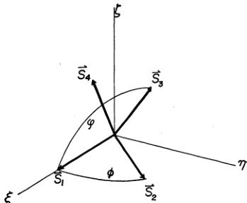
If we choose the \( \xi \) , \( \eta \) , and \( \zeta \) axes so that \( S_{1} \) is parallel to the \( \xi \) axis and \( S_{2} \) is in the \( \zeta \) plane as is shown in Fig. 14, the second summation of eq.

Fig. 14. Definition of \( \xi \) , \( \eta \) , and \( \zeta \) axes.
(11) can be written
\[ \begin{array}{r}{f(\alpha)=\alpha_{2\xi}+\alpha_{3\xi}+\alpha_{4\xi}+\alpha_{2\xi}\alpha_{3\xi}+\alpha_{2\eta}\alpha_{3\eta}+\alpha_{2\xi}\alpha_{4\xi}}\\ {+\;_{2\eta}\alpha_{4\eta}+\alpha_{3\xi}\alpha_{4\xi}+\alpha_{3\eta}\alpha_{4\eta}+\alpha_{3\xi}\alpha_{4\xi},}\end{array} \quad (19) \]
and the conditions in eq. (12) as
\[ \left.\begin{array}{l}\alpha_{2\xi}^{2}+\alpha_{2\eta}^{2}=1\\\alpha_{3\xi}^{2}+\alpha_{3\eta}^{2}+\alpha_{3\xi}^{2}=1\\\alpha_{4\xi}^{2}+\alpha_{4\eta}^{2}+\alpha_{4\xi}^{2}=1\end{array}\right\}. \quad (20) \]
We now introduce Lagrangian multipliers \( \lambda_{2} \) , \( \lambda_{3} \) and \( \lambda_{4} \) and define a function \( F(\alpha) \) as
\[ \begin{array}{r}{F(\alpha)=f(\alpha)-\lambda_{2}(\alpha_{3\xi}^{2}+\alpha_{2\eta}^{2}-1)-\lambda_{3}(\alpha_{3\xi}^{2}+\alpha_{3\eta}^{2}+\alpha_{3\xi}^{3}-1)}\\ {-\lambda_{4}(\alpha_{4\xi}^{2}+\alpha_{4\eta}^{2}+\alpha_{4\xi}^{3}-1).}\end{array} \quad (21) \]
We set the partial derivatives of \( F(\alpha) \) for all \( \alpha \) 's and \( \lambda \) 's equal to zero at the pole of \( f(\alpha) \) . The derivatives for \( \lambda \) 's give eq. (20) and those for \( \alpha \) 's give the following set of equations.
\[ \left(\begin{array}{c c c}{-2\lambda_{2}}&{1}&{1}\\ {1}&{-2\lambda_{3}}&{1}\\ {1}&{1}&{-2\lambda_{4}}\end{array}\right)\left(\begin{array}{c}{\alpha_{2\xi}}\\ {\alpha_{3\xi}}\\ {\alpha_{4\xi}}\end{array}\right)=-\left(\begin{array}{c}{1}\\ {1}\\ {1}\end{array}\right), \quad (22) \]
\[ \left(\begin{array}{c c c}{-2\lambda_{2}\quad1\quad1}\\ {1\quad-2\lambda_{3}\quad1}\\ {1\quad1\quad-2\lambda_{4}}\end{array}\right)\left(\begin{array}{c}{\alpha_{29}}\\ {\alpha_{39}}\\ {\alpha_{49}}\end{array}\right)=0, \quad (23) \]
\[ \left(\begin{array}{c c}{-2\lambda_{3}}&{1}\\ {1}&{-2\lambda_{4}}\end{array}\right)\left(\begin{array}{c}{a_{3\xi}}\\ {a_{4\xi}}\end{array}\right)=0. \quad (24) \]
If we define the determinants of the left sides of eq. (24) and eq. (22) (or eq. (23)) as \( D_{1} \) and \( D_{2} \) , respectively, we can divide the problem into several categories, depending upon the values of \( D_{1} \) and \( D_{2} \) .
(A) \( D_{1} \neq 0 \)
We get \( \alpha_{3}\xi=\alpha_{4}\xi=0 \) immediately from eq. (24) and all the spins must lie in the \( \zeta \) plane.
(A.1) \( D_{2} \neq 0 \)
All spins are collinear in the \( \xi \) direction because \( \alpha_{2\eta}=\alpha_{3\eta}=\alpha_{4\eta}=0 \) from eq. (23). Furthermore, from eq. (20) we get \( \alpha_{2\xi},\alpha_{3\xi},\alpha_{4\xi}=\pm1 \) but obviously only antiferromagnetic alignment of the spins gives the minimum exchange energy.
(A.2) \( D_{2}=0 \)
In order to solve eq. (22), \( \lambda_{4} \) must be \( -\frac{1}{2} \) . Then the conditions \( D_{1}=0 \) and \( D_{2}=0 \) give \( \lambda=-\frac{1}{2} \) , resulting in \( \alpha_{2\eta}=\alpha_{3\eta}=\alpha_{4\eta}=0. \) From eq. (23), which is the same result as in the case of (A.1).
(B) \( D_{1}=0 \)
(B.1) \( D_{2} \neq 0 \)
From eq. (23) all spins must lie in the \( \eta \) plane just as in the case of (A.1). As eq. (22) gives the relation \( (1+2\lambda_{4})\times(1+\alpha_{3\xi})=0 \) and \( 1+2\lambda_{4}\neq0 \) from the conditions \( D_{1}=0 \) and \( D_{2}\neq0 \) , the relation \( \alpha_{3\xi}=-1 \) is obtained. Then, the second equations gives eq. (20) and eq. (24) gives \( \alpha_{4\xi}=0 \) . Thus, all the spins are again in the \( \xi \) direction.
(B.2) \( D_{2}=0 \)
The two conditions \( D_{1}=D_{2}=0 \) result in \( \lambda_{3}=\lambda_{4}=-\frac{1}{2} \) . Using these relations and combining eqs. (22) and (23), the relation \( \lambda_{2}=-\frac{1}{2} \) is obtained. Equations (22), (23) and (24) can be reduced to the following three independent equations.
\[ \left.\begin{array}{l}\alpha_{2\xi}+\alpha_{3\xi}+\alpha_{4\xi}=-1\\ \alpha_{2\eta}+\alpha_{3\eta}+\alpha_{4\eta}=0\\ \alpha_{3\xi}+\alpha_{4\xi}=0\end{array}\right\}. \quad (25) \]
As we have only six eqs. (20) and (25) for 8 unknown quantities, we can introduce two arbitrary parameters, say the angles \( \varphi \) between \( S_{1} \) and \( S_{2} \) , and \( \psi \) between \( S_{1} \) and \( S_{3} \) (see Fig. 13). Then the simultaneous eqs. (20) and (25) can be solved straight forwardly and the solution is listed in Table VI. There, another parameter \( \psi' \) is
Table VI. Solution of eqs. (20) and (25).
| \( \alpha_{3}^{\xi} \) | \( \alpha_{\eta} \) | \( \alpha_{\zeta} \) | |
| \( S_{1} \) | 1 | 0 | 0 |
| \( S_{2} \) | \( \cos \varphi \) | \( \sin \varphi \) | 0 |
| \( S_{3} \) | \( \cos \psi \) | \( -\frac{(1+\cos \varphi)(1+\cos \psi)}{\sin \varphi} \) | \( -\sqrt{\frac{2(1+\cos \psi^{\prime})(1+\cos \psi)(1+\cos \varphi)}{\sin \varphi}} \) |
| \( S_{4} \) | \( \cos \psi^{\prime} \) | \( -\frac{(1+\cos \varphi)(1+\cos \psi^{\prime})}{\sin \varphi} \) | \( \sqrt{\frac{2(1+\cos \psi^{\prime})(1+\cos \psi^{\prime})(1+\cos \varphi)}{\sin \varphi}} \) |
introduced as the angle between \( S_{1} \) and \( S_{4} \) . It is apparent from the first equation in eq. (25) that the condition (13) must be imposed among the angle \( \varphi \) , \( \psi \) and \( \psi' \) . The collinear result in the cases (A.1), (A.2) and (B.1) is included in this case, if we choose \( \varphi=0 \) , \( \psi=180^{\circ} \) ( \( \psi'=180^{\circ} \) ) or \( \varphi=180^{\circ} \) , \( \psi=0^{\circ} \) ( \( \psi'=180^{\circ} \) ) or $ \varphi=180^{\circ}, \psi=180^{\circ}\
\[ \frac{(\boldsymbol{\alpha}_{1}+\boldsymbol{\alpha}_{2})(\boldsymbol{\alpha}_{3}+\boldsymbol{\alpha}_{4})}{|\boldsymbol{\alpha}_{1}+\boldsymbol{\alpha}_{2}||\boldsymbol{\alpha}_{3}+\boldsymbol{\alpha}_{4}|}=-1. \quad (25) \]
It is worthwhile to note that the relation \( \alpha_{1}+\alpha_{2}+\alpha_{3}+\alpha_{4}=0 \) always holds, corresponding to an antiferromagnetic spin configuration, and that the exchange energy density is equal to \( 4NJS^{2}(<0) \) , which is lower than the paramagnetic energy density 0.
References
1) V. L. Sedov: Soviet Physics-JETP 15 (1962) 88.
2) M. Shiga and Y. Nakamura: J. Phys. Soc. Japan 19 (1964) 1743.
3) J. S. Kouvel and J. S. Kasper: J. Phys. Chem. Solids 24 (1963) 529.
4) R. Nathans and S. J. Pickart: J. Phys. Chem. Solids 25 (1964) 183.
5) S. Miyake et al.: J. Phys. Soc. Japan 17B-II (1962) 358.
6) M. Hansen: Constitution of Binary Alloys (McGraw Hill, 1958) p. 666.
7) K. P. Gupta, C. H. Cheng and P. A. Beck: J. Phys. Chem. Solids 25 (1964) 73.
8) T. Nagamiya, K. Yosida and R. Kubo: Advances in Phys. 4 (1955) 1.
9) S. C. Abraham, L. Guttman and J. S. Kasper: Phys. Rev. 127 (1962) 2052.
10) U. Gonser, C. J. Meecham, A. H. Muir and H. Wiedersich: J. appl. Phys. 34 (1963) 2373.
11) Y. Ishikawa, H. Endho and H. Umebayashi: to be published.
12) J. Smit and H. P. J. Wijn: Ferrites (John Wiley 1959) p. 46.
13) C. Kimball, W. D. Gerber and A. Arrott: J. appl. Phys. 34 (1963) 1064.
 p10_0.jpg
 p10_1.jpg
 p11_0.jpg
 p13_0.jpg
 p4_0.jpg
 p4_1.jpg
 p4_2.jpg
 p5_0.jpg
 p5_1.jpg
 p6_0.jpg
 p6_1.jpg
 p8_0.jpg
 p9_0.jpg
 p9_1.jpg